Synopsis

This paper presents a novel explicit reconstruction method for magnetic resonance-based electrical properties tomography (EPT). We derive the dbar equation for the electric field that incorporates the variation of the magnetic field along the longitudinal axis. This new dbar equation allows an explicit reconstruction of the electrical properties even when the magnetic field varies along that axis. We also propose an iterative reconstruction procedure that solves the dbar equation by the Cauchy–Pompeiu formula and updates EP values in each step. The proposed method correctly reconstructed EPs even in the case that the magnetic field and EPs vary along the longitudinal direction.

Introduction

Methods

By taking the $$$(x+iy)$$$- and $$$z$$$-components of time-harmonic Maxwell’s equations, we have

$$\bar{\partial}E_{z} = \omega\mu_{0}H^{+}+\partial_{z}E^{+},\quad 4\partial H^{+} = -\omega\kappa E_{z}, \quad\partial_{z} H^{+}=\omega\kappa E^{+},$$

where $$$\partial\equiv(\partial_{ x}-i\partial_{y})/2,\,\bar{\partial}\equiv(\partial_{x}+i\partial_{y})/2,\,H^{+}\equiv(H_{x}+iH_{y})/2,\,E^{+}\equiv(E_{x}+iE_{y})/2$$$ and $$$\kappa\equiv\epsilon-i\sigma/\omega$$$. $$$\omega_{0}/2\pi$$$ is the Larmor frequency and $$$\sigma$$$ and $$$\epsilon$$$ are the conductivity and the permittivity, respectively. Eliminating $$$E^{+}$$$ from these equations yields

$$\bar{\partial}E_{z}+\frac{\partial_{z}^{2}H^{+}}{4\partial H^{+}}E_{z} = \omega\mu_{0}H^{+}-\frac{\partial_{z}^{2}H^{+}}{\omega}\partial_{z}\left(\frac{1}{\kappa}\right).$$

According to Vekua¹¹, we introduce an integral operator, $$$T$$$, satisfying $$$\bar{\partial}T[f]=f$$$. It can be shown, then, that the above equation is equivalent to the following equation:

$$\bar{\partial}\left(E_{z}\exp\left(T\left[\frac{\partial_{z}^{2}H^{+}}{4\partial H^{+}}\right]\right)\right)=\left(\omega\mu_{0}H^{+}-\frac{\partial_{z}^{2}H^{+}}{\omega}\partial_{z}\left(\frac{1}{\kappa}\right)\right)\exp\left(T\left[\frac{\partial_{z}^{2}H^{+}}{4\partial H^{+}}\right]\right).$$

This is the dbar equation for $$$E_{z}\exp([A])$$$ where $$$A\equiv\partial_{z}^{2}H^{+}/(4\partial H^{+})$$$ and its solution is explicitly given by the Cauchy–Pompeiu formula⁹. This new dbar equation includes $$$\partial_{z}H^{+}$$$ and thus is valid even when 2D approximation does not hold. If it holds that $$$\partial_{z}H^{+}=0$$$, the equation is reduced to $$$\bar{\partial}E_{z}=\omega\mu_{0}H^{+}$$$ that we utilized in our previous method. Based on the above, we can construct the reconstruction procedure as follows: First, we assume that $$$\partial_{z}\kappa=0$$$ and reconstruct $$$E_{z}$$$ directly by the following formula:

$$E_{z}(\zeta)=\frac{1}{2\pi i} \int_{\partial D} \frac{-4\partial H^{+}/(\omega\kappa)\exp(T[A](\zeta^{\prime})-T[A](\zeta))}{\zeta^{\prime}-\zeta}d\zeta^{\prime}-\frac{1}{\pi}\iint_{D}\frac{\omega\mu_{0}H^{+}\exp(T[A](\zeta^{\prime})-T[A](\zeta))}{\zeta^{\prime}-\zeta}dx^{\prime}dy^{\prime},$$

where $$$\zeta\equiv x+iy$$$, and calculate $$$\kappa$$$ from $$$E_{z}$$$ by Faraday's law. Then, we correct the dbar equation by using previously obtained $$$\kappa$$$ and solve it again. We note that no iteration is needed if $$$\partial_{z}\kappa=0$$$ holds near the region of interest even in the case that the magnetic field varies along the longitudinal direction.

We evaluated the proposed method by numerical simulations using an FEM simulator, COMSOL Multiphysics (COMSOL Inc.) and by a phantom experiment using 3 T MR scanner (Siemens, Magnetom Prisma). In numerical simulations, we constructed two simulation models (model 1 and 2) that shared the same shape but had different lengths as shown in figure 1. We compare the proposed method with our previous method with 2D approximation and no iterative correction.

Results and Discussion

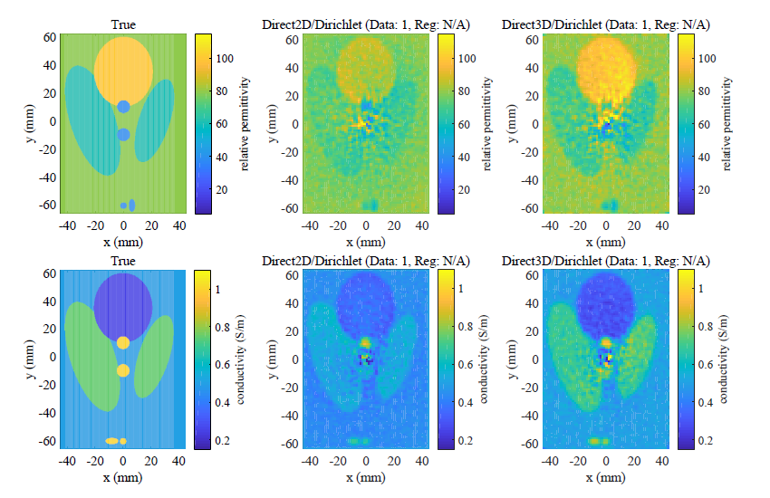
Figure 2 shows the reconstruction results of model 1 when 1% of Gaussian noise was added. The previous method with 2D approximation yields lower estimations whereas the proposed method reconstructed more precisely. This is because the proposed method correctly accounted for the variation of $$$H^{+}$$$ along the $$$z$$$-direction. Figure 3 shows the reconstructed maps in simulation 2 when the same noise was added. In this case, the proposed method with no correction still yields lower estimations due to the assumption that $$$\partial_{z}\kappa=0$$$. However, only a single iteration sufficiently corrected the results. Figure 4 shows the experimental phantom and the reconstructed conductivity maps. It can be shown that the proposed method successfully distinguished three cylindrical regions with higher conductivity.

The reconstructed maps have spot-like artifacts in low electric-field regions⁴ and regularization methods should be adopted to alleviate them. Validations using human anatomical models are also our future work.

Conclusion

In this paper, we presented a novel EPT reconstruction method based on the dbar equation of the electric field that accounts for the variation of the magnetic field along the longitudinal axis. Unlike our previous method that corrected the effect of this magnetic field variations in an iterative manner, the proposed method can explicitly reconstruct EPs that are constant in the longitudinal direction near the region of interest even when the magnetic field varies along that axis. We also proposed an iterative reconstruction procedure that solves the dbar equation directly and updates EP values in each step to retrieve three-dimensionally distributed EPs. Numerical simulations and phantom experiments showed that the proposed method correctly reconstructed EPs even in the case that the magnetic field and EPs vary along the longitudinal axis.

Acknowledgements

References

1. Katscher U, van den Berg CAT. Electric properties tomography: Biochemical, physical and technical background, evaluation and clinical applications. NMR Biomed. 2017;30(8):1–15.

2. Joines WT, Zhang Y, et al. The measured electrical properties of normal and malignant human tissues from 50 to 900 MHz. Med. Phys. 1994;21(4):547–550.

3. Collins CM, Liu S, and Smith MB. SAR and B1 Field Distributions in a Heterogeneous Human Head Model within a Birdcage Coil. Magn. Reson. Med. 1998;40(6):847–856.

4. Hafalir FS, Oran OF, et al. Convection-reaction equation based magnetic resonance electrical properties tomography(cr-MREPT). IEEE Trans. Med. Imag. 2014;33(3):777–793.

5. Ammari H, Kwon H, et al. Magnetic-resonance-based reconstruction method of conductivity and permittivity distribution at Larmor frequency. Inverse Problems. 2015;31(10):105001.

6. Hong R, Li S. 3-D MRI-Based Electrical Properties Tomography Using the Volume Integral Equation Method. IEEE Trans. Microw. Theory Tech. 2017;65(12):4802–4811.

7. Balidemaj E, van den Berg CAT, et al. CSI-EPT: A Contrast Source Inversion Approach for Improved MRI-Based Electric Properties Tomography. IEEE Trans. Med. Imag., 2015;34(9):1788–1796.

8. Arduino A, Zilberti L, et al. CSI-EPT in presence of RF-shield for MR-coils. IEEE Trans on Med Imag. 2017;36(7):1396–1404.

9. Nara T, Furuichi T, Fushimi M. An explicit reconstruction method for magnetic resonance electrical property tomography base on the generalized Cauchy formula. Inverse Problems. 2017;33(10):105005.

10. Fushimi M, Nara T. A Boundary-Value-Free Reconstruction Method for Magnetic Resonance Electrical Properties Tomography Based on the Neumann-type Integral Formula over a Circular Region. SICE JCMSI. 2016;10(6):571–578.

11. Vekua I. Generalized Analytic Functions. Pergamon Press, 1962.

12. Insko EK, Bolinger L. Mapping of the radiofrequency field. J. Magn. Reson. 1993;103(1):82–85.