5052
Inverse problem approach to cr-MREPT1Dept of EEE, Bilkent University, Ankara, Turkey
Synopsis
The convection-reaction partial differential equation (PDE) based algorithm for Magnetic Resonance Electrical Properties Tomograpy, cr-MREPT, does not suffer from internal boundary artifacts but has the Low Convective Field (LCF) artifact. The cr-MREPT PDE is rearranged such that H1+ is the unknown variable and the coefficients depend on the EPs. The EPs are iteratively adjusted to minimize the difference between calculated and measured H1+. The method can be applied to a Region-of-Interest without considering the whole object. Conductivity reconstructions for simulation objects and also for an agar phantom demonstrate that the proposed method does not suffer from boundary and LCF artifacts.
Introduction
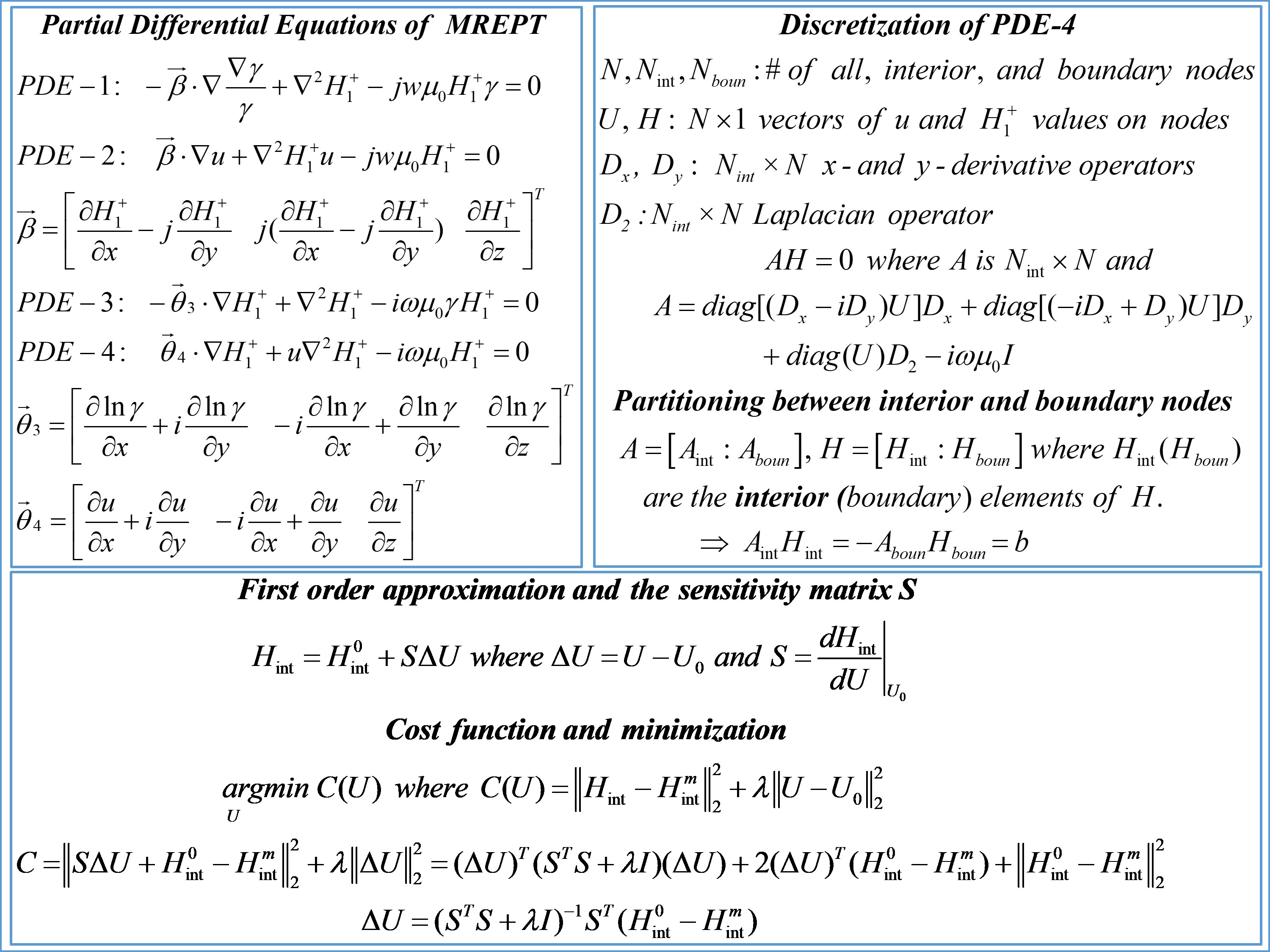
The partial differential equations (PDEs) of MREPT are shown in Figure-1. PDE-1 and PDE-2 are alternative equations where admittivity $$$\gamma=\sigma+i\omega\epsilon$$$ and impedance $$$u=\frac{1}{\gamma}$$$ are the unknown variables, respectively. The coefficients of these equations depend on the measured $$$H_1^+$$$ and the solution of either one with specified EPs on the boundary of a Region-of-Interest (ROI) yields the EPs inside. PDE-2 is also called the cr-MREPT equation1. In contrast to this “direct” approach, with the “inverse problem approach” EPs are adjusted (iteratively) so that solution of the forward problem approaches the measured $$$H_1^+$$$. Alternative formulations for the forward problem are PDE-3 and PDE-4 where the unknown variable is $$$H_1^+$$$ and the coefficients are EP dependent. In this study the “inverse problem approach” is implemented using PDE-4, called Inv-crMREPT, and is compared with the “direct” solution, cr-MREPT.Methods
The ROI is discretized by a regular Cartesian mesh. $$$U$$$ and $$$H$$$ are the vectors of nodal impedance and $$$H_1^+$$$ values respectively. PDE-4 is discretized at each interior node to obtain the set of linear algebraic equations $$$AH=0$$$, and one can solve for the interior values $$$H_{int}$$$, given the boundary values $$$H_{boun}$$$, as explained in Figure-1. Difference between this calculated $$$H_{int}^{calc}$$$ and measured $$$H_{int}^{m}$$$ is minimized iteratively to obtain $$$U$$$. Figure-1 defines the minimization problem where $$$\lambda$$$ is Tikhonov regularization parameter. At each iteration the sensitivity matrix $$$S$$$ (Jacobian) is calculated to approximate $$$H_{int}$$$ around the previously found EP distribution $$$U_0$$$ which is taken as uniform for the first iteration.
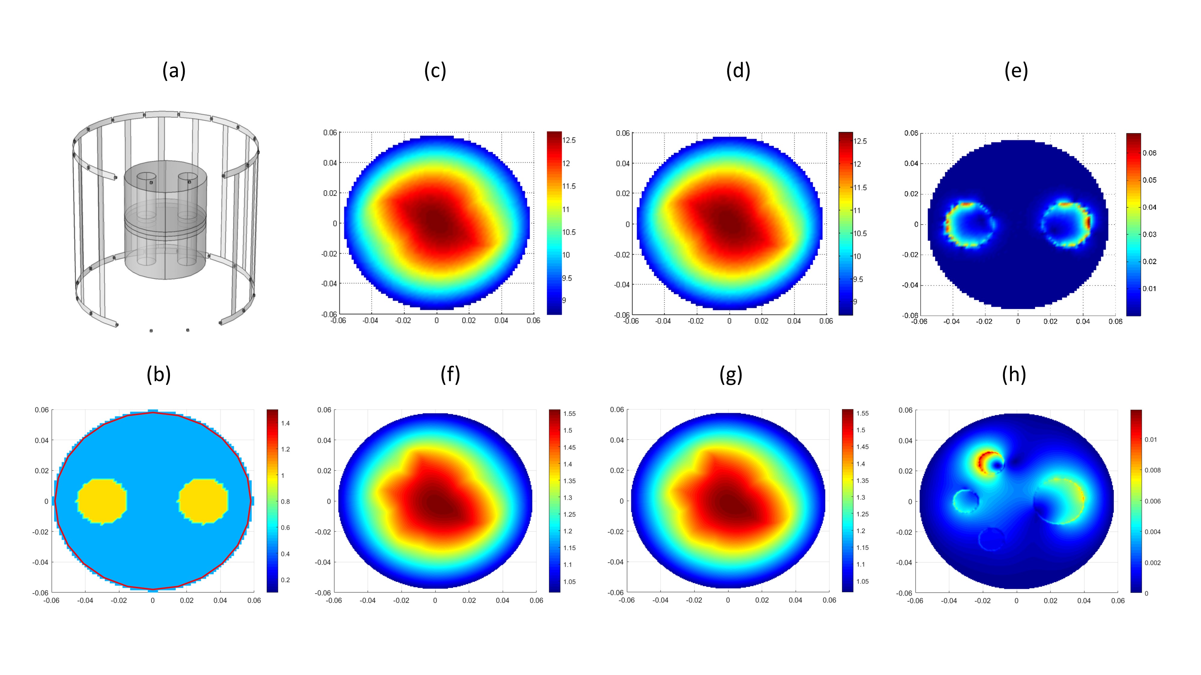
For std-MREPT $$$\gamma=\frac{\triangledown^2H_1^+}{i\omega\mu_0H_1^+}$$$ is used2. For cr-MREPT, PDE-2 is regularized by adding an artificial diffusion term3,4 ,discretized, and solved for $$$U$$$ in one step without iterations. 3D cylindrical simulation phantom placed in a birdcage RF coil is shown in Figure-2. For 2D simulations the object is placed in a uniform applied rotating RF magnetic field. Normalized RMS errors, $$$NRMSE_{\sigma}=\frac{\parallel \sigma_{calc}-\sigma_{real}\parallel_2}{\parallel \sigma_{real}\parallel_2}$$$ and $$$NRMSE_{H_{int}}=\frac{\parallel H_{int}^{calc}-H_{int}^{m}\parallel_2}{\parallel H_{int}^{m}\parallel_2}$$$ are used for performance assessment. Experiments are conducted with an agar phantom with the same dimensions and EP properties as the 3D simulation phantom. bSSFP and Bloch-Siegert sequences are used for $$$H_1^+$$$ phase and magnitude mapping respectively.
Results
Figure-2 shows for the 3D and 2D simulation phantoms that using the simulated $$$H_1^+$$$ data on the ROI boundary as a Dirichlet BC and the actual EPs in the ROI, the $$$H_1^+$$$ obtained in the ROI by solving PDE-4 is very similar to the simulated $$$H_1^+$$$ except for some minor (less than 0.5%) differences on the sharply varying anomaly boundaries (The ROI was selected to cover the central slice $$$\pm$$$5 slices for 3D application). These observations are in line with the uniqueness theorem proved by Ammari et al5.
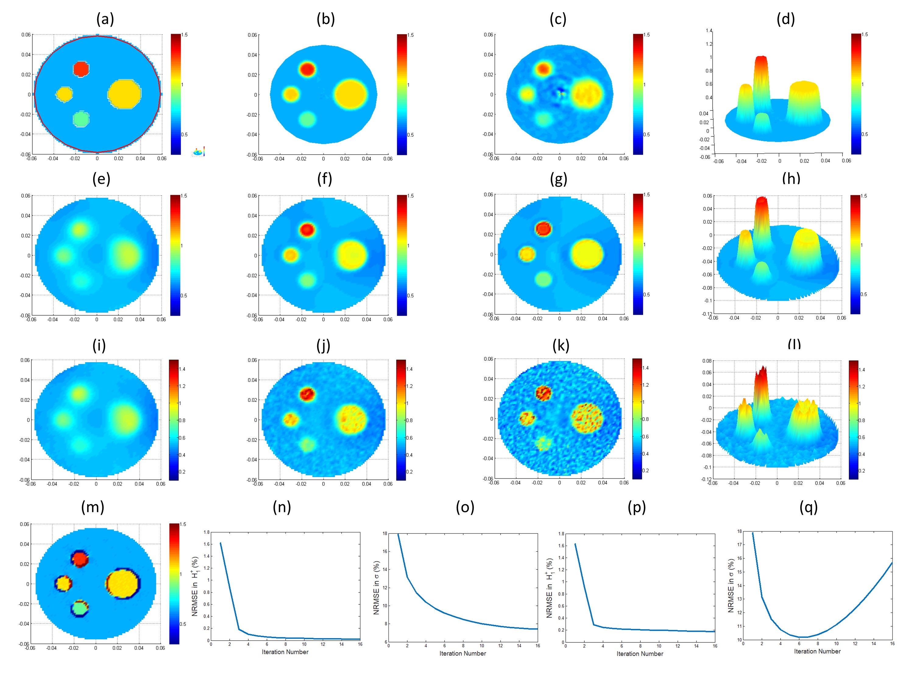
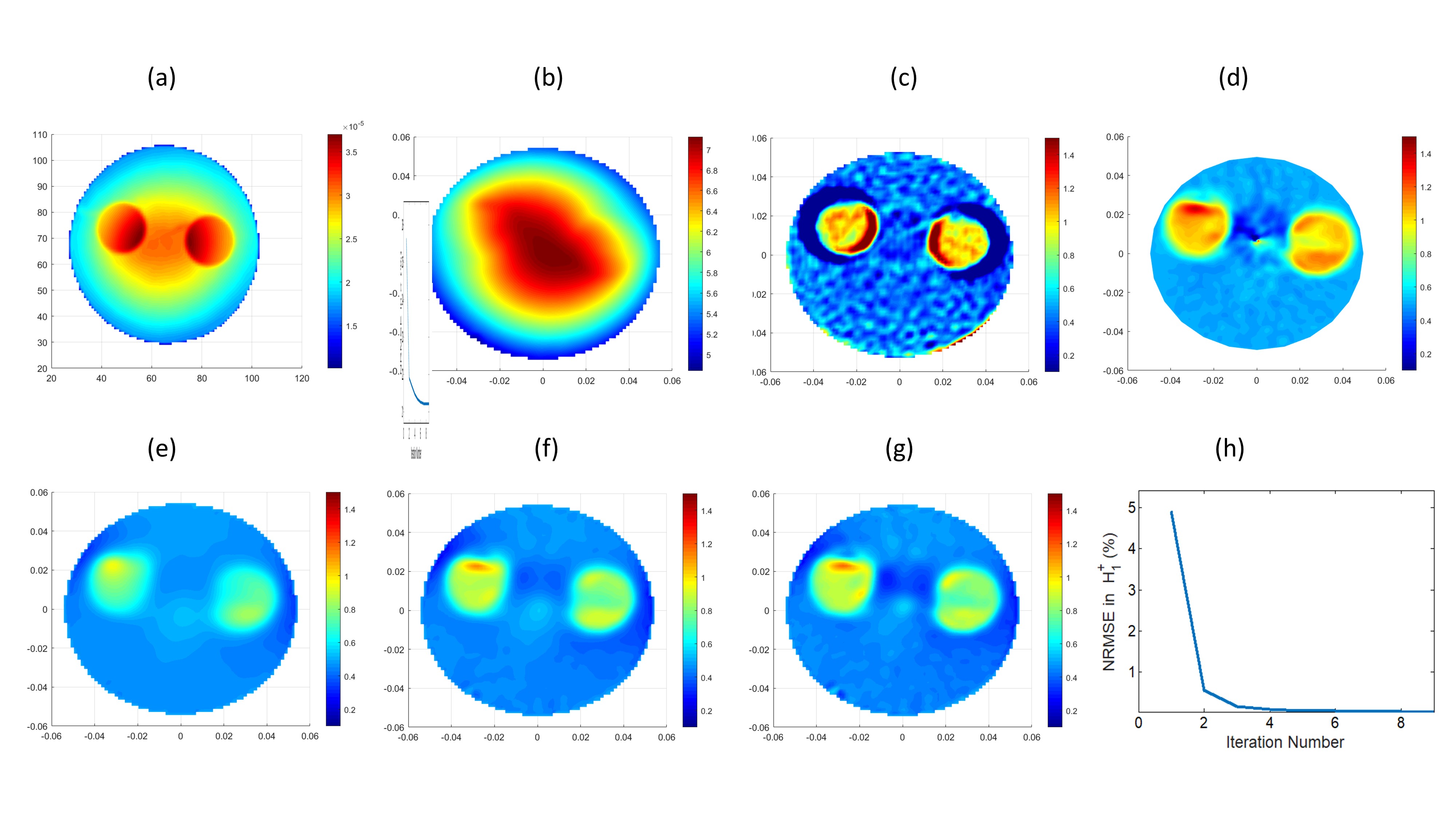
Figure-3 shows the conductivity reconstructions for the 2D simulation phantom. std-MREPT has the notorious internal boundary artifacts. cr-MREPT has no boundary artifacts but the LCF-artifact1 appears when Gaussian noise is added (SNR = 300) to the simulated $$$H_1^+$$$. With Inv-crMREPT after the 6th iteration $$$NRMSE_{H_{int}}$$$ does not decrease further whereas $$$NRMSE_{\sigma}$$$ still improves. With additive noise, a divergent behavior starts for $$$NRMSE_{\sigma}$$$ after the 6th iteration. In any case, Inv-crMREPT does not suffer from boundary and LCF artifacts. Each iteration of 2D Inv-crMREPT takes 45 seconds for a ROI with 4709 nodes (pixel size of 1.5mm).
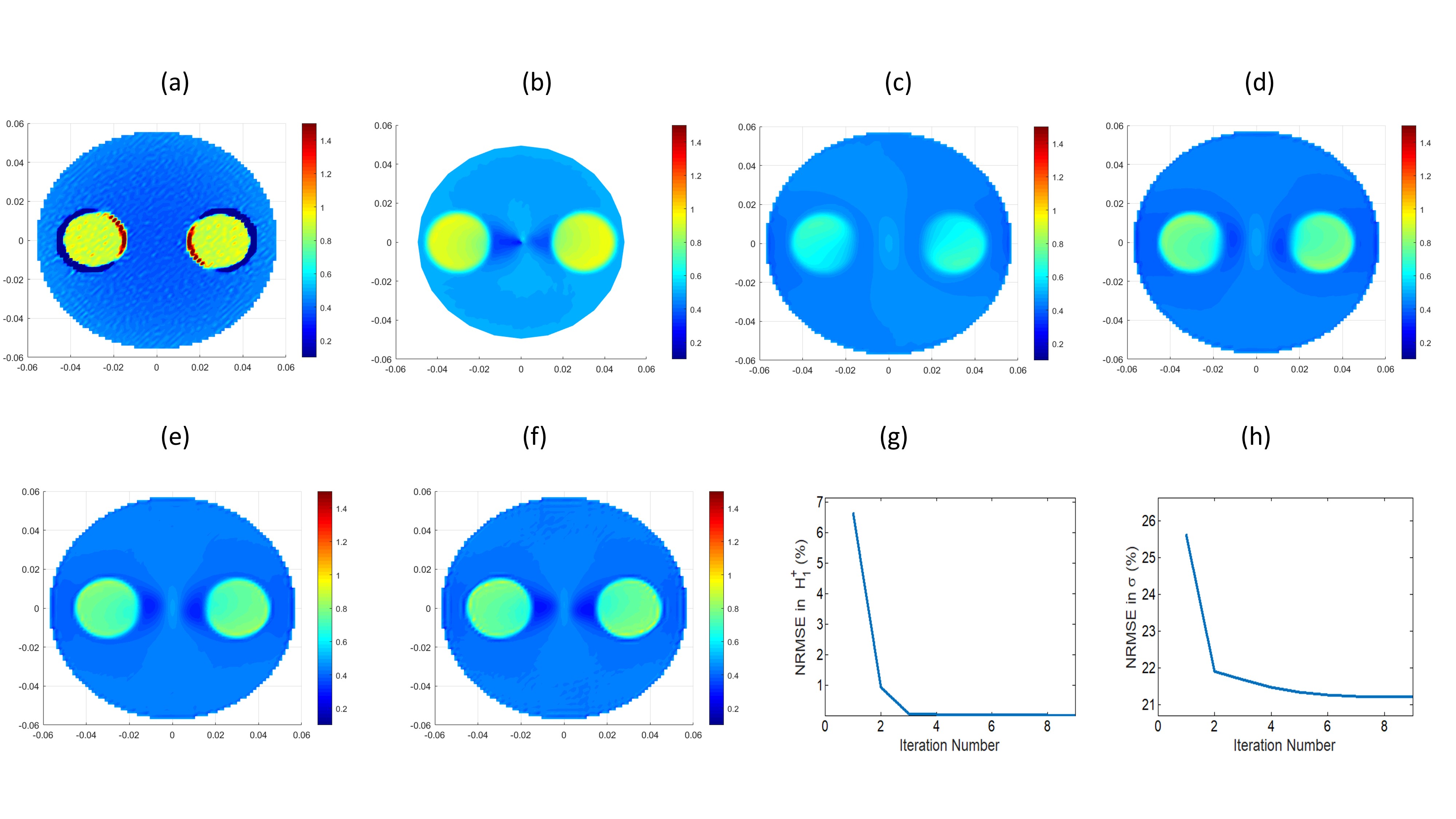
Central slice reconstructions for the 3D simulation phantom and the experimental phantom are shown in Figures 4 and 5, respectively. In both cases, Inv-crMREPT does not have boundary and LCF artifacts. However some inaccuracies observed in conductivity values may be due to the fact that we have used the 2D version of PDE-4 for reconstruction.
Discussion
Inv-crMREPT makes a second order approximation to the cost function and approximates the Hessian by $$$S^TS$$$. We have achieved convergence starting from a uniform distribution. In their inverse approach Ammari et al have used steepest descent optimization, and have developed an adjoint based fast method to find the gradient of the cost function5. However they need a good initial estimate of the EP distribution. The “inverse problem approach” used by Borsic et al6 and the “model based” approach used by Ropella et al7 are limited to the phase-only formulation of conductivity reconstruction. The scattering model based approach of Leijsen et al8 handles the object as a whole and has to be modified to handle a ROI independently. Implementation of Inv-crMREPT in a 3D ROI must be done using the 3D version of PDE-4, which of course needs more memory and solution time.Conclusion
The “inverse problem approach” proposed in this study and the resulting iterative implementation, called Inv-crMREPT, provides conductivity reconstructions which are free from boundary and LCF artifacts. 3D implementation of the method is necessary for more accuracy, and is under way.
Acknowledgements
This study is supported by Tubitak grant 114E522. We thank Safa Ozdemir for his contribution in the MR experiments.References
1. Hafalir FS, Oran OF, Gurler N, Ider YZ. Convection-Reaction Equation Based Magnetic Resonance Electrical Properties Tomography (cr-MREPT). IEEE Trans Med Imaging. 2014;33(3):777-793. doi:10.1109/tmi.2013.2296715.
2. Katscher U, Kim DH, and Seo JK. Recent Progress and Future Challenges in MR Electric Properties Tomography. Computational and Mathematical Methods in Medicine, Volume 2013, Article ID 546562, 11 pages. doi:10.1155/2013/546562
3. Li C, Yu W, Huang SY. An MR-Based Viscosity-Type Regularization Method for Electrical Property Tomography. Tomography. 2017;3(1):50-59. doi:10.18383/j.tom.2016.00283.
4. Gurler N and Ider YZ. Gradient-Based Electrical Conductivity Imaging Using MR Phase. Magnetic Resonance in Medicine, 2016;77(1):137-150. doi: 10.1002/mrm.26097
5. Ammari H, Kwon H, Lee Y, Khang K, Seo J. Magnetic resonance-based reconstruction method of conductivity and permittivity distributions at the Larmor frequency. Inverse Probl. 2015;31(10):105001. doi:10.1088/0266-5611/31/10/105001
6. Borsic A, Perreard I, Mahara A, Halter RJ. An Inverse Problems Approach to MR-EPT Image Reconstruction. IEEE Trans Med Imaging 2016;35:244–256. doi: 10.1109/TMI.2015.2466082.
7. Ropella KM, Noll DC. A Regularized, Model-Based Approach to Phase-Based Conductivity Mapping Using MRI. Magn Reson Med. 2016;78(5):2011-2021. doi:10.1002/mrm.26590.
8. Leijsen RL, Brink WM, van den Berg CAT, Webb AG, and Remis RF. 3-D Contrast Source Inversion-Electrical Properties Tomography. IEEE Trans Med Imaging, 2018, 37:2080-2089. doi:10.1109/TMI.2018.2816125
Figures