5051
A dual constraints-based approach to electrical conductivity imaging using MR phase1University of Electronic Science and Technology of China, Chengdu, China, 2Southern Medical University, Guangzhou, China, 3Philips Healthcare, Guangzhou, China
Synopsis
Electrical conductivity imaging of tissue can potentially provide electrical property information of tissues. Here, we proposed
Introduction
Electrical conductivity imaging is a non-invasive method to retrieve the distribution of conductivity which is significantly different between normal tissue and tumor1, 2. The conventional method depends on the assumption that electrical properties distribution is locally constant3. However, this assumption is not satisfied in practice, such as the human head, which would cause boundary artifact. Moreover, the Laplacian operator which is sensitive to noise makes the results worse4. To solve these problems, the gradient-based method and inverse method were improved5, 6. Here, we proposed a dual constraints-based conductivity imaging method which includes the gradient of conductivity and uses MR transceive phase.Theory
In previous studies, a gradient-based partial differential equation between transceive phase $$$\phi$$$ and conductivity $$$\sigma$$$ is derived from Maxwell’s equation. The equation includes the gradient of conductivity, as follow:
$$\triangledown\phi\cdot\triangledown\rho+\triangledown^{2}\phi\rho-2\omega \mu_{0}=0 (1)$$
Where $$$\rho=1/\sigma$$$, $$$\omega$$$ is angular frequency and $$$\mu_{0}$$$ is magnetic permeability. The partial differential can be represented by the central difference method, and then for an image matrix, equation (1) can be written as a linear system equation $$$A\rho=b$$$. This equation is solved by least squares regularized by total variation and wavelet transform, as follow:
$$\widehat{\rho}=argmin_{\rho}\frac{1}{2}\parallel A \rho-b \parallel_2^2+\lambda_{1}\parallel\rho \parallel_{tv}+\lambda_{2}\parallel W\rho \parallel_{1} (2)$$
Where $$$\widehat{\rho}$$$ is the optimal conductivity solution, $$$W$$$ is a wavelet transform, $$$tv$$$ is total variation. $$$\lambda_{1}$$$ and $$$\lambda_{2}$$$ are regularization parameter respectively. These regularizations can reduce the boundary spurious oscillation and suppress noise. Equation (2) is solved by split Bregman method7.
Method
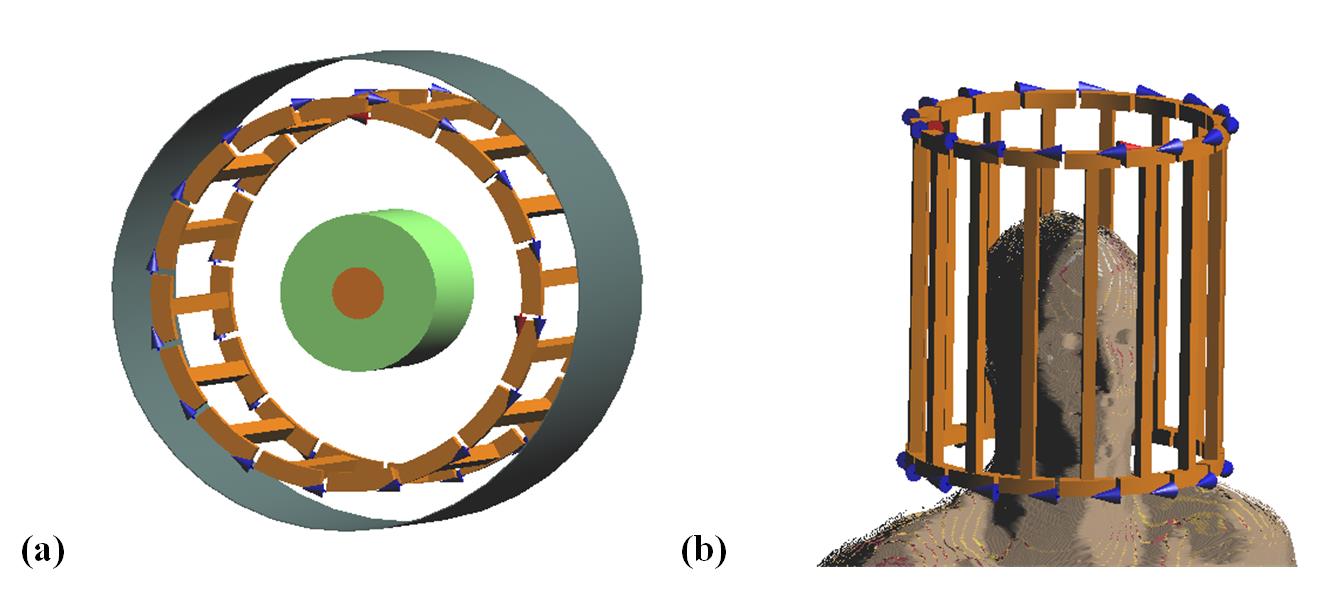
Simulations: Numerical simulations were performed using a Finite-Difference Time-Domain (FDTD) based software (SEMCAD X. 14.6, Zurich Switzerland). The simulation model includes quadrature birdcage coil, cylindrical phantom and human brain model (Duke Model, Virtual family) as shown in Figure 1. The phantom consisted of the outer and inner compartment that assigned different conductivity values, which is 1.0 (s/m), 1.5 (s/m) respectively, the simulation was performed at 128MHz. By using quadrature excitation model, the phase of $$$B_1^+$$$ and $$$B_1^-$$$ was got from the software, and then add these phases to get transceive phase.
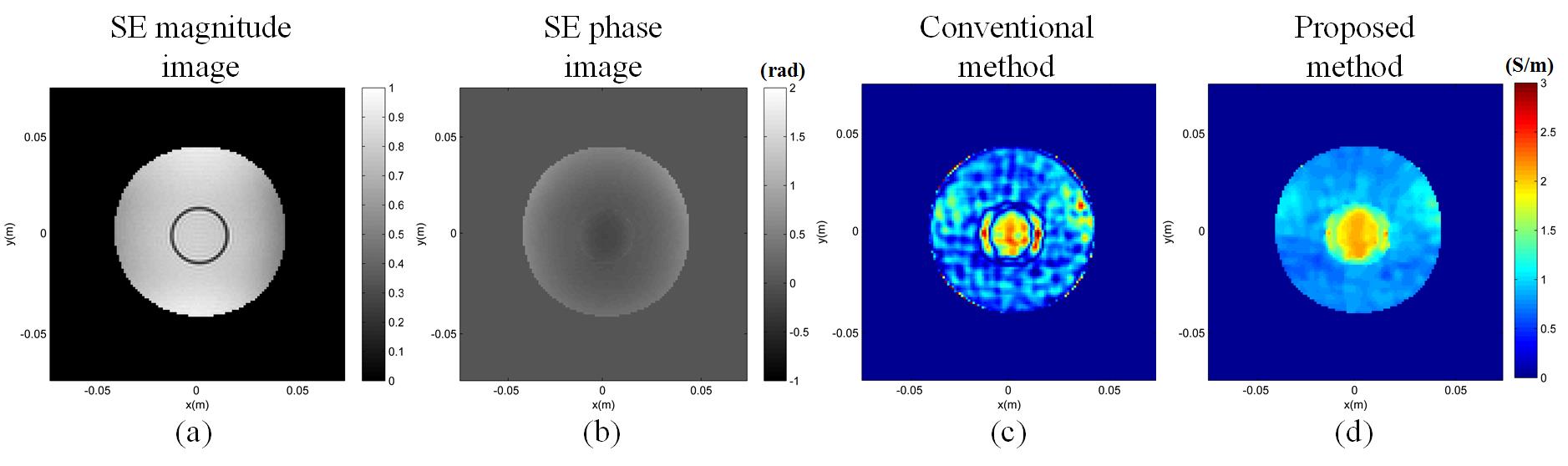
Experimental: The phantom was cylindrical with a diameter of 90mm and a length of 120mm. It consisted of an inner and outer compartment which was similar to the simulation phantom. These two parts were separated by tube, the measured conductivity values of these two parts were 2.01 (s/m), 0.97 (s/m). The experiment was conducted on a 3.0T MR scanner (Philips Achieva, Best, The Netherlands), quadrature volume coil as transmits coil and 8-channel receive coil was used for reception. To measure the transceive phase, spin echo (SE) sequence was applied.
Results
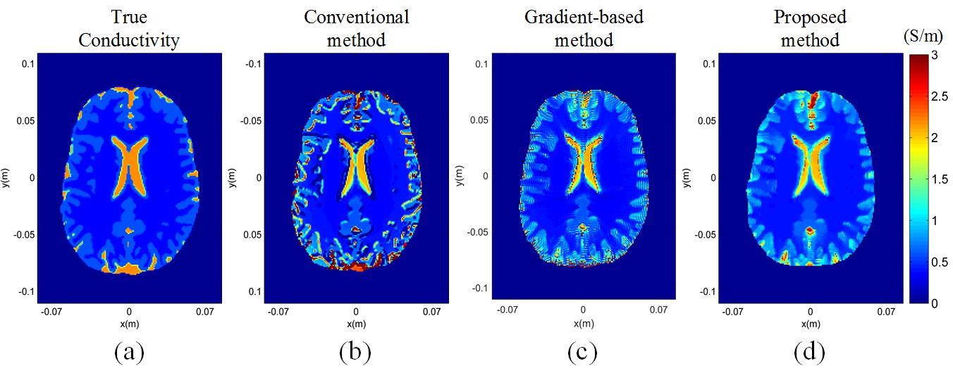
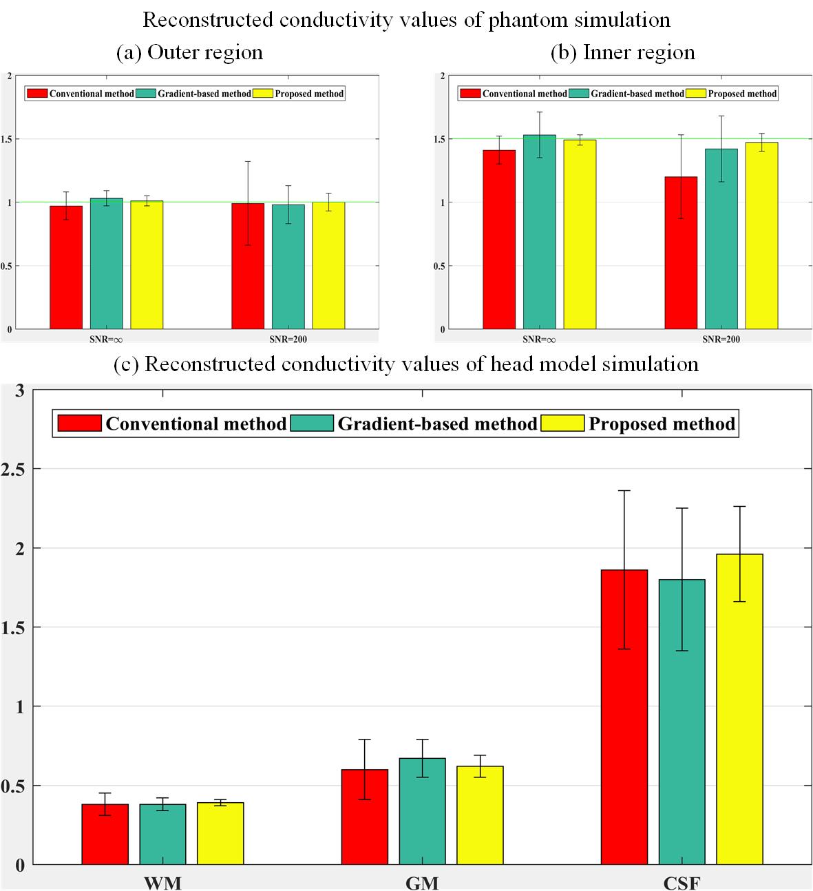
Figure 2 shows the reconstructed conductivity maps of simulation phantom. It is observed that the proposed method mitigates boundary artifacts and alleviate oscillations in the gradient-based method. Moreover, the proposed method still achieves a good reconstructed result in the case of noise. Figure 3 presents the results of head model simulation. The proposed method can reconstruct a clearer brain structure. Figure 4 is the results from the phantom experiment, the mean conductivity value of the proposed method is 1.90(S/m), 0.83(S/m) which is close to the measured value. In Figure 5, the average and standard deviation of conductivity values indicate that the proposed method improves the accuracy of conductivity images.Discussion
Previous studies on electrical conductivity imaging were influenced by boundary artifacts and transceiver phase assumption. In this study, a dual constraints-based conductivity imaging method based solely on the MR transceive phase was used to retrieve the distribution of conductivity. The proposed method exploits total variation and wavelet transform regularization terms to reduce the effect of noise and improve the accuracy of conductivity estimates. By applying this method to phantom experiment, the scanning time is short and the quality of reconstructed results was significantly improved, but the parameter of this technique should be easy to choose.Conclusion
A dual constraints-based conductivity imaging method is a robust and accurate method to retrieve conductivity distribution, it does not need locally constant assumption and transceive phase assumption, therefore, it has the potential to the clinical applications.Acknowledgements
This work was supported by the National key research and development program under grant 2016YFC0104003, the National Natural Science Foundation of China under grants 61471188,81871437, 61628105, 81501541, U1708261, the Natural Science Foundation of Guangdong Province under grants 2016A030313577, and the Program of Pearl River Young Talents of Science and Technology in Guangzhou under grant 201610010011.References
1. W. T. Joines, Y. Zhang, C. Li, and R. L. Jirtle, The measured electrical properties of normal and malignant human tissues from 50 to 900 MHz. Med. Phys. 1994; 21(4): 547-550.
2. U. Katscher, T. Voigt, C. Findeklee, P. Vernickel, K. Nehrke, and O. Dossel, Determination of electric conductivity and local SAR via B1 mapping. IEEE Trans. Med. Imaging 2009; 28(9): 1365-1374.
3. J. K. Seo, M. O. Kim, J. Lee, N. Choi, et al. Error analysis of nonconstant admittivity for MR-based electric property imaging. IEEE Trans. Med. Imaging. 2012; 31(2): 430-437.
4. H. Wen. Noninvasive quantitative mapping of conductivity and dielectric distributions using RF wave propagation effects in high-field MRI. In Proc. SPIE, San Diego, USA, 2003; 5030: 471-477.
5. K. M. Ropella, D. C. Noll. A regularized, model-based approach to phase-based conductivity mapping using MRI. Magn. Reson. Med. 2016; 78(5): 2011-2021.
6. N. Gurler, Y. Z. Ider. Gradient-based electrical conductivity imaging using MR phase. Magn. Reson. Med. 2017; 77(1): 137-150.
7. W. Yin, S. Osher, D. Goldfarb, J. Darbon. Bregman Iterative Algorithms for l1-Minimization with Applications to Compressed Sensing. SIAM J. Imaging Sci. 2008; 1(1): 143-168, 2008.
Figures