5049
Compensation of lead-wire magnetic field contributions in MREIT experiment using image segmentation: a phantom study1School of Biological and Health Systems Engineering, Arizona State University, Tempe, AZ, United States, 2Department of Physics, University of Florida, Gainesville, FL, United States, 3Philips Research, Huston, TX, United States, 4Department of Biochemistry and Molecular Biology, University of Florida, Gainesville, FL, United States
Synopsis
For the measurement of current-induced phase using MRI, the effect of stray magnetic fields caused by the current carrying wire on images must be minimized prior to reconstruction of the current density. In this study, we report a method which can effectively remove the effect of lead wire magnetic fields interference during MREIT measurements. Results from phantom experiments and numerical simulations demonstrate the feasibility of the method, which can be used to correct for lead effects when measuring current density in human transcranial direct current stimulation (tDCS) measurements using magnetic resonance electrical impedance tomography (MREIT).
INTRODUCTION:
In tDCS, small currents are injected through a pair of surface electrodes attached on the head1. Presently, distributions of tDCS current within the head are estimated using subject-specific computational models2-3. However, these models employ literature conductivities for head tissues and real distributions may be quite different. Therefore, MREIT techniques have recently been used to estimate current density distributions directly4-6. In MREIT, one component of the magnetic flux density (in the direction of the main magnetic field of the scanner, z) induced due to external current injection is collected using a MRI scanner. The acquired MREIT signal can be expressed as7-8,
$$B_z(\mathbf{r})= \frac{\mu_0}{4\pi}\int_{\Omega}\frac{(y-y^{'})J_x(\mathbf{r'})-(x-x^{'})J_y(\mathbf{r^{'}})}{\mid\mathbf{r}-\mathbf{r^{'}}\mid^3}d\mathbf{r^{'}}+B_{z,\mathcal{L}}~~~~(1)$$
where, $$$\mathbf{r}$$$ and $$$\mathbf{J}=[J_x,J_y,J_z]$$$ are position and current density vectors respectively. The first term of (1) describes magnetic flux density produced by the external current injection inside the head domain $$$\Omega$$$7. The second term describes magnetic flux density caused by lead wires . This can be minimized if wires are aligned with the $$$z$$$-direction8. However, in practical tDCS measurements, aligning wires along the direction is problematic, so it is crucial to account for the magnetic field of the wires. The effect of wires is explored in this study using a hemispherical phantom.
METHODS:
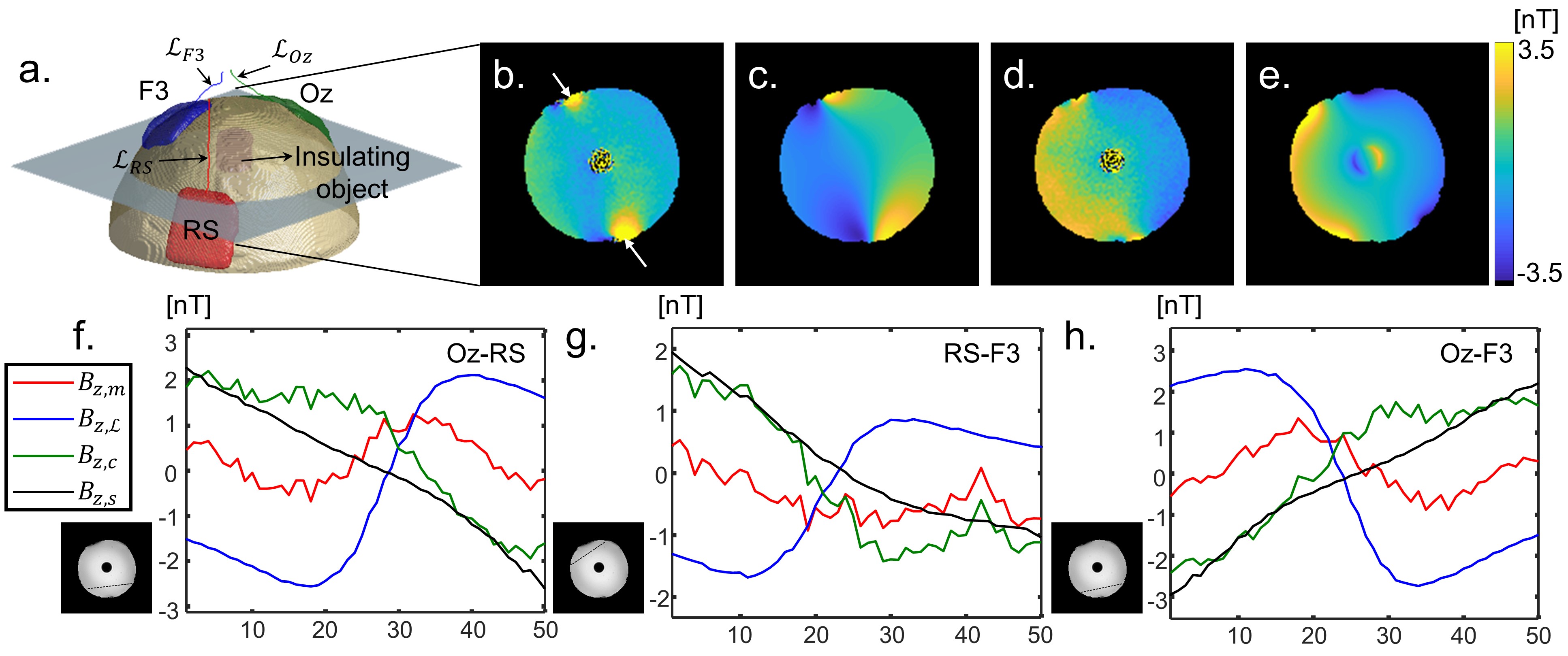
Experiment set-up: All data were measured using a 32-channel head coil in a 3.0 T Philips MRI scanner. (Barrow Neurological Institute, Phoenix, Arizona). The phantom contained agar-gel (conductivity of 1 S/m). A non-conductive acrylic rod anomaly was placed inside the phantom (Fig-1a). Three carbon electrodes (F3, RS, Oz) were attached to the phantom surface (Fig. 1a). Wires were encapsulated with silicone tubing (Tygon 3350 Sanitary Silicone Tubing, Saint Gobain, Paris, France) to enable MR detection. We performed MREIT imaging at 1.5 mA current amplitude, using a MR-safe tDCS stimulator (Neuroconn, Ilmenau, Germany). A multi gradient echo sequence5 was used to collect 3 slices of $$$B_{z,m}$$$ (subscript $$$m$$$ denotes measured data). The parameters used in the sequence were, TR/TE = 50/7ms, NE = 10, ES = 3ms, NEX = 24, Matrix size 160x160, FOV = 240 mm, Slice thickness, 5 mm. A set of T1-weighted images with matrix size, 240x240x140 resulting in 1mm3 isotropic resolution, was also collected during the same experimental session.
Stray magnetic field correction: A three-dimensional tube mask was created from the high resolution T1-weighted images. In order to segment the tube, the ‘flood-fill’ algorithm in ScanIP (Synopsys Inc., Mountain View, CA, USA) software was used. For some cases, morphological dilation operations were used to close the segmented mask. Segmented tube masks were then exported to MATLAB (The MathWorks. Inc., Natick, MA, USA). Wire trajectories were determined from mask centroids (Fig. 1a). Stray magnetic field ($$$\mathbf{B}_\mathcal{L}=[B_{x,\mathcal{L}},B_{y,\mathcal{L}},B_{z,\mathcal{L}}]$$$) was then computed as7,
$$\mathbf{B}_{\mathcal{L}}(\mathbf{r}) = \frac{I\mu_0}{4\pi}\int_{\mathcal{L}}\mathbf{\hat{a}}(\mathbf{r^{'}})\times \frac{\mathbf{r}-\mathbf{r^{'}}}{\mid\mathbf{r}-\mathbf{r^{'}}\mid^3}dl^{'} ~~~~ (2)$$
where $$$I$$$ is amplitude of current and $$$\mathbf{\hat{a}}(\mathbf{r^{'}})$$$ is the unit vector in the direction of the current flow at $$$\mathbf{r}^{'} \in \mathcal{L}$$$. Computed $$$B_{z,\mathcal{L}}$$$ fields were subtracted from acquired $$$B_{z,m}$$$ data to obtain corrected magnetic fields $$$B_{z,c}$$$.
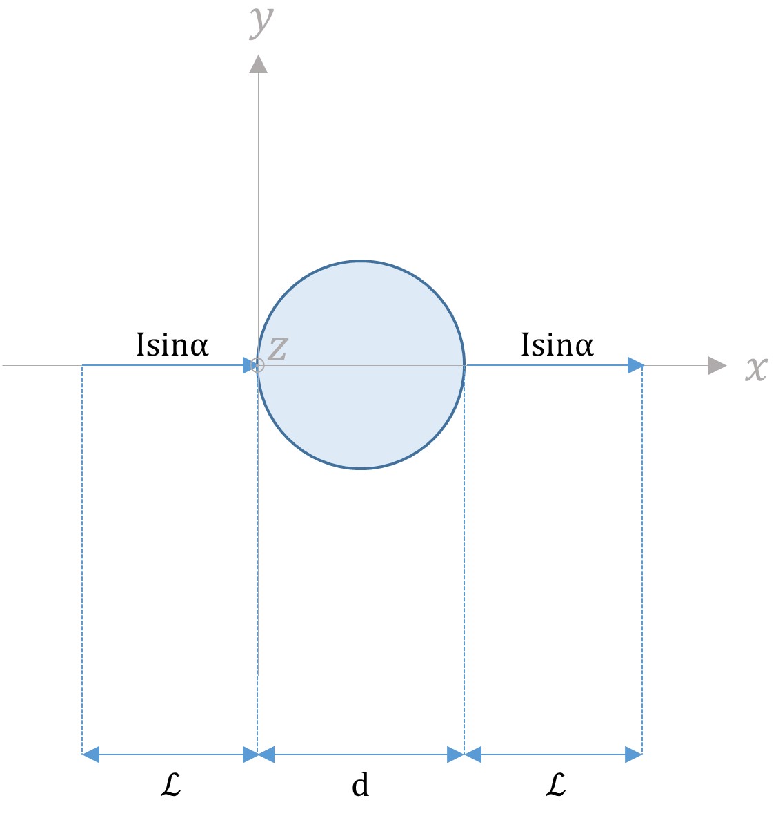
Validation: Contributions to $$$B_{z,\mathcal{L}}$$$ were analyzed analytically as (Fig 2),
$$\begin{cases}B_{z,\mathcal{L}} = \frac{\mu_0I\sin\alpha}{4\pi y}\left(\frac{\mathcal{L}+x}{\sqrt{(\mathcal{L}+x)^2+y^2}}-\frac{\mathcal{L}+x}{\sqrt{x^2+y^2}}+\frac{\mathcal{L}+d-x}{\sqrt{(\mathcal{L}+d-x)^2+y^2}}-\frac{d-x}{\sqrt{(d-x)^2+y^2}}\right) \\B_{z,\mathcal{L}}(x=d/2,y) = \frac{\mu_0I\sin\alpha}{2\pi y}\left(\frac{\mathcal{L}+d/2}{\sqrt{(\mathcal{L}+d/2)^2+y^2}}-\frac{d/2}{\sqrt{(d/2)^2+y^2}}\right)\end{cases}~~~~(3)$$
Results were also verified against numerical simulations. Simulated $$$B_{z,s}$$$ data, were obtained by solving the Laplace equation within the hemisphere alone using the COMSOL-MATLAB interface (COMSOL Inc., Burlington, MA, USA). The conductivity of the simulated hemisphere was set to the gel conductivity (1 S/m) and anomaly conductivity was set to 0 S/m. The data was then computed from calculated current density distributions using the Biot-Savart law.
Results:
Figure 1(b) shows the 5th-echo of the center slice of $$$B_{z,m}$$$ data from current flow through the Oz-RS pair. The arrow indicates strong $$$B_{z,s}$$$ effects nearby wires. The computed stray $$$B_{z,s}$$$ flux density for same electrode montage is shown in figure 1(c). As can be seen in figure 1(d), wire effects were effectively removed after stray field subtraction. Simulated $$$B_{z,s}$$$ and profile plots are shown in figure 1(e-h) for comparison, with profiles matching well in terms of scale. Differences between corrected and simulated profiles may be due to conductivity variations within the phantom.DISCUSSION:
Corrections were only applied on one echo of the multi echo data, but optimum use of the data would involve producing a weighted sum of echoes to maximize SNR5. In future work, we will correct individual echo data for wire-created stray field prior to optimization.CONCLUSIONS:
These results confirm that stray fields may produce large effects on tDCS-related magnetic flux densities6. Methods that use wire detection and modeling may be appropriate to correct these images before use in reconstructions of current density4.Acknowledgements
This work was supported by award RF1MH114290 to RJS.References
1. Nitsche M A and Paulus W. Excitability changes induced in human motor cortex by weak transcranial direct current stimulation. J. Physiol., 2000; 527(3): 633-9.
2. Sadleir R J, Vannorsdall T D, Schretlen D J et al. Transcranial direct current stimulation (tDCS in a realistic head model. NeuroImage, 2010; 51(4):1310-18.
3. Datta A, Baker J M, Bikson M et al. Individual model predicts brain current flow during transcranial direct-current stimulation treatment in responsive stroke patient. Brain Stimul., 2011; 4(3):169-74.
4. Kwon O I, Sajib S Z K, Sersa I et al. Current density imaging during transcranial direct current stimulation using DT-MRI and MREIT: algorithm development and numerical simulations. IEEE Trans. Biomedical Eng., 2016; 63(1): 168-75.
5. Kasinadhuni A K, Indahlastari A, Chauhan M et al. Imaging of current flow in the human head during transcranial electrical therapy. Brain Stimul., 2017; 10(4):764-72.
6. Göksu C, Hanson L G, Siebner H R et al. Human in-vivo brain magnetic resonance current density imaging (MRCDI). NeuroImage, 2018; 171:26-39.
7. Lee B I, Oh S H, Woo E J et al. Three-dimensional forward solver and its performance analysis for magnetic resonance electrical impedance tomography using recessed electrodes. Phys. Med. Biol. 2003; 48(13):1971-86.
8. Sajib S Z K, Katoch N, Kim H J et al. Software toolbox for low-frequency conductivity and current density imaging using MRI. IEEE Trans. Biomedical Eng., 2017; 64(11): 2505-14.
Figures