Purpose

Chemical Exchange Saturation Transfer (CEST) can detect the presence of proteins, metabolites, and other macromolecular structures. At ultra-high field strengths, CEST effects produce distinct dips in the Z-spectrum and can be quantified by non-linear least squares (NLLS) fitting of a multi-Lorentzian model [1]. At clinical field strengths, broad and coalesced peaks make NLLS sensitive to noise and measurement errors. Moreover, pixel-wise NLLS fitting is computationally expensive and unsuitable for online reconstruction of CEST contrast images. Here, we investigate the use of neural networks for fast quantification of CEST pool parameters from noisy Z-spectra acquired at 3T.

Methods

Spectrally selective CEST contrast was acquired at B0=3T with 3D-GRE snapshot CEST (1.7x1.7x3 mm resolution, Tacq=6 min 35sec) with 4s of pulsed low-power presaturation (Gauss pulses, B1=0.6µT, tp=20.48ms) applied at 54 variably-spaced offsets between +/–100ppm [2,3]. Data were acquired in 3 healthy subjects (Siemens Prisma) and in 1 brain tumor patient (Siemens Verio PET/MR). Brain matter Z-spectra were manually segmented and de-noised using principle component analysis (first 7 components retained) [2,3]. De-noised Z-spectra were fitted pixel-wise by NLLS with a 4-pool Lorentzian model [1] of direct water saturation, semisolid magnetization transfer (MT), amide (APT), and NOE pools. Noisy Z-spectra from 3 slices in different brain regions of one subject were used as input for a 3-layer deep neural network (NN, 400 neurons in total) with the NLLS fitted Lorentzian pool parameters from de-noised Z-spectra as target values. The dataset was divided randomly into training (70%), validation (15%), and test sets (15%) used to avoid overfitting. Trained with about 3000 iterations, the NN was applied to noisy Z-spectra from other slices in the same volunteer, two additional healthy subjects, and one brain tumor patient.

Results

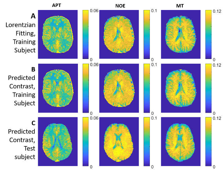
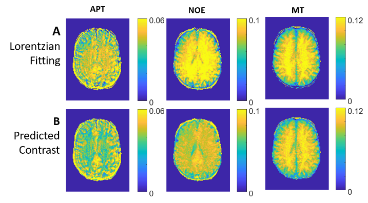
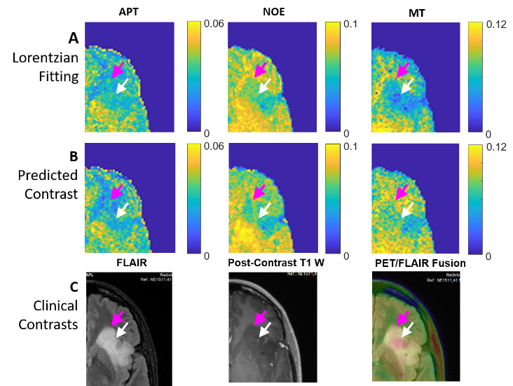
Lorentzian NLLS fitting of de-noised, 3D Z-spectra takes approximately 6.5 minutes for 14 slices using parallel computation. Training the NN on 3 slices from a single subject took 5.8 minutes, but applying the NN to predict 4-pool Lorentzian model parameters in 14 slices takes only 2 seconds. Figure 1 compares quantitative CEST maps in a representative test slice from NLLS fitting and the NN prediction in the training subject and a test subject. The predicted contrasts have the same amplitude, spatial distribution, and smoothness as the de-noised NLLS fitting results. Similar results are seen in untrained data from the test subject. Figure 2 shows results from a subject with motion during the scan. NLLS fitting results exhibit disrupted contrast and elevated signal. However, the NN prediction is more robust to motion errors, with the pool sizes similar to Figure 1 and the expected contrasts in healthy tissues. Figure 3 shows predicted CEST contrast in a brain tumor patient. NLLS fitting results in better contrast between normal gray and white matter, tumor core (white arrow) and the surrounding edema. However, the NN prediction highlights more subtle details, such as increased APT and NOE signals coinciding with slightly increased FET uptake (pink arrow).

Discussion & Conclusion

In low SNR data typically acquired at clinical field strengths, stable results from NLLS fitting of multi-Lorentzian models require careful consideration of boundary and initial conditions. This proof-of-concept study demonstrates that a NN trained on one subject can be successfully applied to estimate CEST pool parameters in another subject, and also yields reasonable results in pathology, with a 95% reduction in computing time. This approach can be used to estimate initial conditions in a NNLS fit, or for fast online calculation of quantitative CEST images. While surprisingly consistent results were obtained in healthy subjects with training on just a few slices from one volunteer, there are many possibilities for further research. The NN can still be optimized, and its properties and learned features further investigated. The NN prediction yields different contrast in the brain tumor data, which has lower SNR than the training dataset. Predicted CEST contrast may improve if more healthy subjects and patients are included in training.

Acknowledgements

Max Planck Society; German Research Foundation (DFG, grant ZA 814/2-1, support to MZ); European Union Horizon 2020 research and innovation programme (Grant Agreement No. 667510, support to MZ, AD).