Synopsis

In vivo CEST MRI data can include contributions from a vast array of metabolites, mobile proteins and peptides, and immobile macromolecules amongst others. Detecting which components are present in any given dataset is a major challenge. Here, as a first start to address the problem, we have used a machine learning approach to classify a CEST dataset acquired from brain metabolite phantoms. The classifier was successful in all cases and was shown to be robust to a moderate level of noise. The results demonstrate this is a promising technique that could potentially quantify molecular contributions in vivo.

Introduction

CEST MRI is an emerging technique for the molecular imaging of endogenous compounds.^1-2 CEST is based on using radiofrequency (RF) irradiation to label MR sensitive nuclei (e.g., protons) in low concentration solute molecules. If these protons physically exchange to the solvent pool (e.g., bulk water), the RF label is also transferred to the solvent. Prolonged or repeated labelling results in multiple label-transfer instances and thus the cumulative effect of labelled protons in the water pool can be several orders of magnitude larger than the concentration of the solute protons. Therefore, the CEST process allows the detection of low concentration solute molecules via the bulk water signal with enhance sensitivity.

CEST experiments are commonly performed by acquiring a saturation spectrum (Z-spectrum) over the proton resonance frequency range.³ In addition to the bulk water, in vivo data contain several other endogenous signals. These signals include metabolites,^4-7 mobile proteins and peptides,^8-9 molecules undergoing reversible binding,¹⁰ and immobile tissue components.^11-12 The relative contributions of these depend on the RF saturation pulse sequence parameters, such as B₁, saturation time and interpulse spacing. Separating out all the contributions or detecting which of the components is changing in a disease therefore is a major hurdle in CEST studies.

In recent years, machine learning has generated great interest due to its ability to extract meaningful patterns from complex data.¹³ Both supervised learning (relating data features to observations) and unsupervised (finding hidden characteristics in the data) approaches may be applicable to CEST MRI data. Here, we used supervised machine learning to train a model for classifying CEST data acquired from 11 brain metabolite phantoms and a mixture of these metabolites based on their brain concentration. As a first step, this approach can be useful for rapidly and autonomously detecting the presence of CEST agents in a set of images.

Materials and Methods

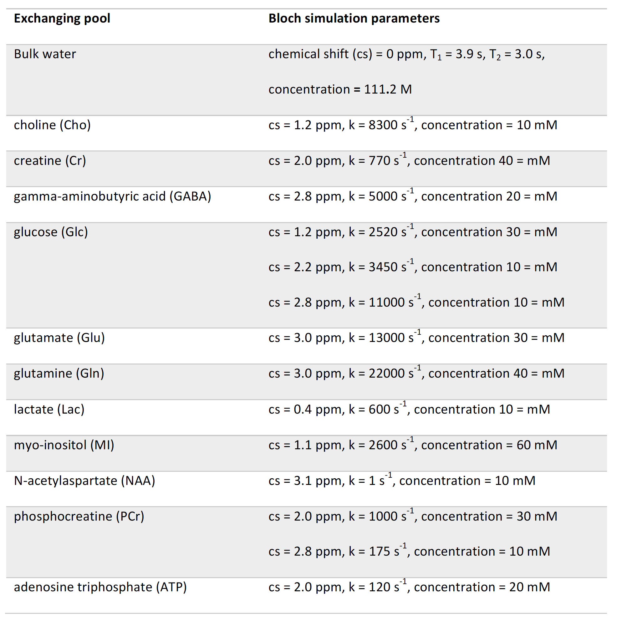
CEST training data for a selection of 11 brain metabolites was generated using the Bloch-McConnell equations¹⁴ with additional Rician noise (approx. 1000 training sets for each metabolite). The simulation parameters for each pool are displayed in Table 1.

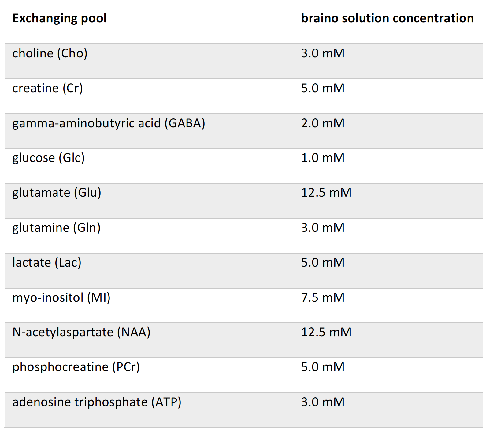
For testing experimental data, the brain metabolites shown in Table 1 were dissolved in phosphate buffered saline (PBS) at concentrations of 10 mM and the pH adjusted to 7.2. Each solution was placed in a 5 mm NMR tube and scanned in a 17.6 T vertical bore scanner (Bruker, Ettlingen, Germany) at 37°C. CEST experimental data were acquired using a 7 s continuous wave (CW) saturation pulse with an amplitude of 3 μT. A braino phantom in PBS (pH = 7.2) was also made using the concentrations given in Table 2.

For machine learning, a random forest model with 100 trees were trained using the python machine learning library scikit-learn.¹⁵ Each training set consisted of the simulated spectra (including noise) and the associated MTR asymmetry spectrum.³ The estimator was cross-validated on a randomized sub-sample of the simulated data with further noise added. The individual metabolite phantoms and braino phantom were then assessed.

Results and Discussion

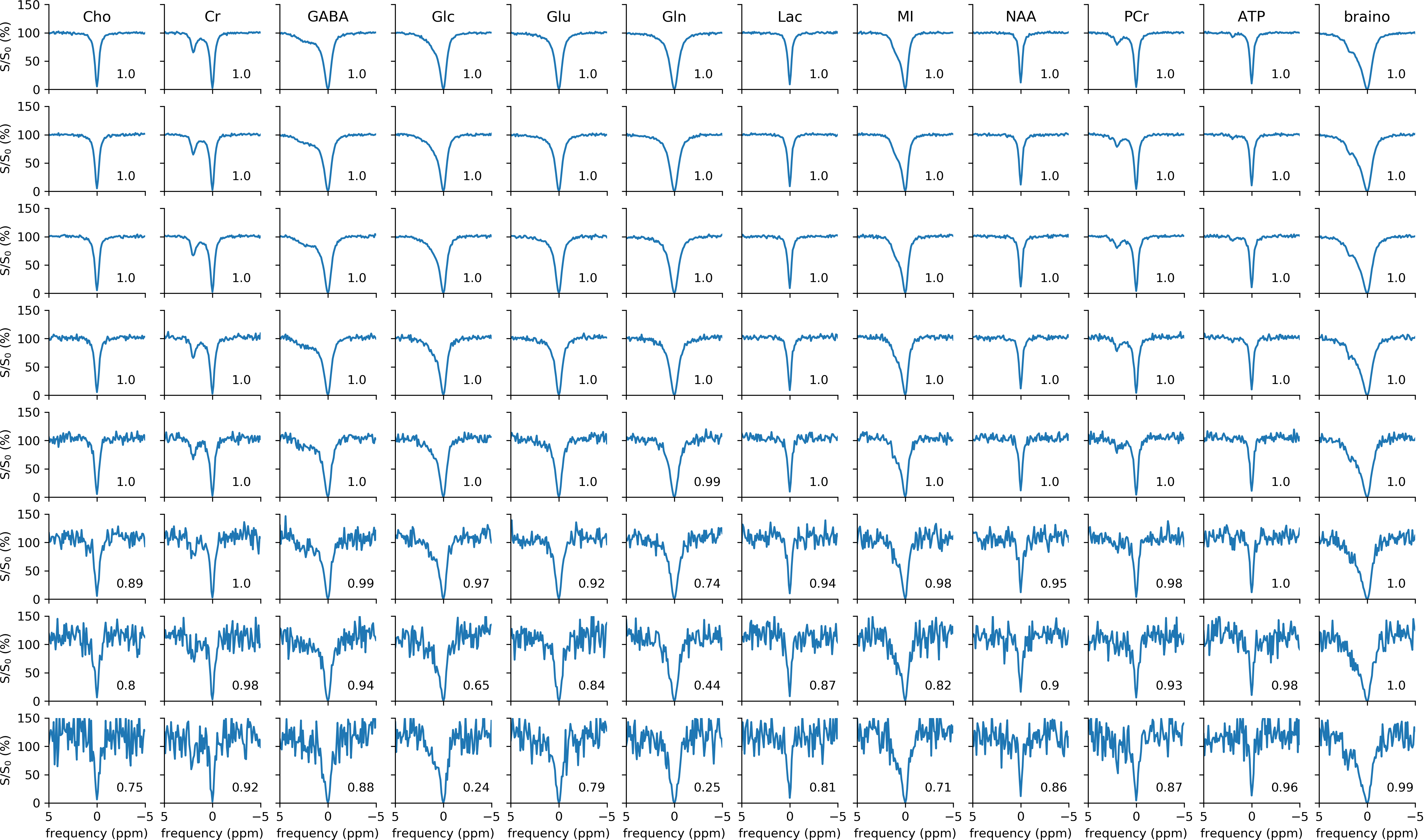
The performance of the classifier on the randomized training data with different noise levels is shown in Figure 1. The results show that the algorithm performed perfectly with for all datasets with noise set to 2.5 standard deviations and a minimum accuracy (f1-score¹⁶) of 0.99 when the standard deviation of the noise was 5. When higher levels of noise were added, the classifier did better with some metabolite spectra compared to others. For instance, the model was able to classify all metabolites except Glc and Gln at higher than 70% accuracy at the highest noise level. We speculate that the poor performance with Glc and Gln at very high noise is due to the similar spectral appearance from fast exchanging protons between 1 to 3 ppm.

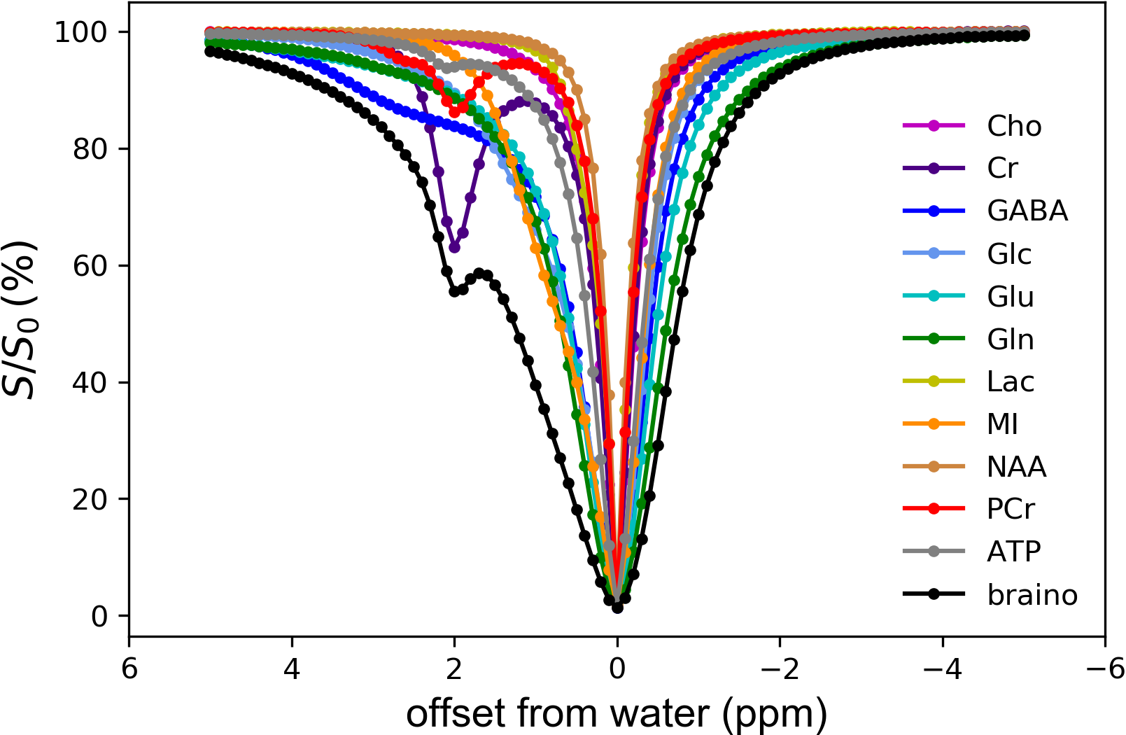
Next, the hypothesis function generated by the classifier was fit to the experimental data from individual phantoms and the combined braino data (Figure 2). All the experimental data was classified accurately via the model developed here. Although it is relatively easy to distinguish the creatine, phosphocreatine, and GABA datasets visually, other datasets are more challenging. The results here show a machine learning approach can rapidly and autonomously classify similar looking spectra with high accuracy. The high accuracy was maintained with even moderately noisy data.

Conclusion

Acknowledgements

References

1. Ward KM, Aletras AH, Balaban RS. A new class of contrast agents for MRI based on proton chemical exchange dependent saturation transfer (CEST). J Magn Reson 2000;143:79-87.

2. van Zijl PCM, Yadav NN. Chemical exchange saturation transfer (CEST): what is in a name and what isn't? Magn Reson Med 2011;65:927-948.

3. Bryant RG. The dynamics of water-protein interactions. Annu Rev Biophys Biomol Struct 1996;25:29-53.

4. Cai K, Haris M, Singh A, Kogan F, Greenberg JH, Hariharan H, Detre JA, Reddy R. Magnetic resonance imaging of glutamate. Nat Med 2012;18:302-306.

5. Haris M, Cai K, Singh A, Hariharan H, Reddy R. In vivo mapping of brain myo-inositol. Neuroimage 2011;54:2079-2085.

6. Kogan F, Haris M, Singh A, Cai KJ, Debrosse C, Nanga RPR, Hariharan H, Reddy R. Method for High-Resolution Imaging of Creatine In Vivo Using Chemical Exchange Saturation Transfer. Magn Reson Med 2014;71:164-172.

7. Chen L, Zeng H, Xu X, Yadav NN, Cai S, Puts NA, Barker PB, Li T, Weiss RG, van Zijl PCM, Xu J. Investigation of the contribution of total creatine to the CEST Z-spectrum of brain using a knockout mouse model. NMR Biomed 2017;30.

8. Zhou J, Lal B, Wilson DA, Laterra J, van Zijl PC. Amide proton transfer (APT) contrast for imaging of brain tumors. Magn Reson Med 2003;50:1120-1126.

9. Zhou J, Payen JF, Wilson DA, Traystman RJ, van Zijl PCM. Using the amide proton signals of intracellular proteins and peptides to detect pH effects in MRI. Nat Med 2003;9:1085-1090.

10. Yadav NN, Yang X, Li Y, Li W, Liu G, Zijl PC. Detection of dynamic substrate binding using MRI. Sci Rep 2017;7:10138.

11. Wolff SD, Balaban RS. Magnetization transfer contrast (MTC) and tissue water proton relaxation in vivo. Magn Reson Med 1989;10:135-144.

12. van Zijl PCM, Jones CK, Ren J, Malloy CR, Sherry AD. MRI detection of glycogen in vivo by using chemical exchange saturation transfer imaging (glycoCEST). Proc Natl Acad Sci USA 2007;104:4359-4364.

13. Jordan MI, Mitchell TM. Machine learning: Trends, perspectives, and prospects. Science 2015;349:255-260.

14. McConnell HM. Reaction Rates by Nuclear Magnetic Resonance. J Chem Phys 1958;28:430-431.

15. Pedregosa F, Varoquaux G, Gramfort A, Michel V, Thirion B, Grisel O, Blondel M, Prettenhofer P, Weiss R, Dubourg V. Scikit-learn: Machine learning in Python. J Mach Learn Res 2011;12:2825-2830.

16. Powers DM. Evaluation: from precision, recall and F-measure to ROC, informedness, markedness and correlation. J Mach Learn Tech 2011;2:37-63.