4985
Insights from the Configuration Model theory accelerate Bloch simulations for dictionary-based T2 mapping1Department of Diagnostic and Interventional Radiology, Technical University of Munich, Munich, Germany, 2Munich School of Bioengineering, Technical University of Munich, Munich, Germany
Synopsis
Muscle water T2 has been proposed as an imaging biomarker of disease activity in neuromuscular diseases. 2D multi-echo spin-echo sequences have been used for muscle T2 mapping with known limitations including the sensitivity to transmit B1 inhomogeneities. Confounding effects on the T2 quantification can be removed by matching the experimental signal with pre-simulated theoretical signal decay curves obtained by Bloch simulations. However, up to now it is unclear what discretization over the slice profile is sufficient to determine a meaningful dictionary. The purpose of this work was to utilize the configuration model in order to determine a minimal number of z-location necessary for the simulation and applies the technique for T2 mapping of in vivo thigh musculature data.
Purpose:
Muscle water T2 has been proposed as an imaging biomarker of disease activity in patients with neuromuscular diseases1-3. 2D multi-echo spin-echo (MESE) sequences have been used for muscle T2 mapping with known limitations including the sensitivity to transmit B1 inhomogeneities1. Bloch simulations and extended phase graph (EPG) techniques have been applied on 2D MESE data to remove the effects of transmit B1 inhomogeneities4,5. Both rely on a dictionary containing signal decay curves for certain T2/B1 value combinations and a subsequent matching step of the experimental data with the simulated values to determine an unbiased T2 value. Bloch simulations are superior to EPG in simulating more complex magnetization pathways as EPG can only take precomputed slice profiles4. However, Bloch simulations require computational expensive simulations of the magnetization for a certain number of spatial locations. Up to now it is unclear how many z-locations are necessary for the generation of MESE dictionaries. The configuration model (CM) has been proposed to describe the magnetization based on dephasing states6. This work applies knowledge obtained by the CM to determine a minimal number of z-locations necessary for simulating a correct signal evolution. The technique is motivated by simulations and applied in the in-vivo T2 mapping of thigh musculature.Methods:
Theory
For simulation, a sequence is discretized into N time intervals of free precession with the same gradient moment p along slice selection direction, followed by instantaneous pulses7. Following the CM, the magnetization can be described with 2N+1 configuration states over a real-space periodicity interval of 2pi/p (~25cm)6. Consequently, the magnetization is fully described in real-space when performing the Bloch simulation at 2N+1 z-locations in slice direction (this defines a required spatial sampling density). However, the slice profile is more narrow than the periodicity interval and therefore only a thinner slab needs to be simulated resulting in less z-locations. If only the overall magnetization is desired, this number can be reduced further.
Simulations
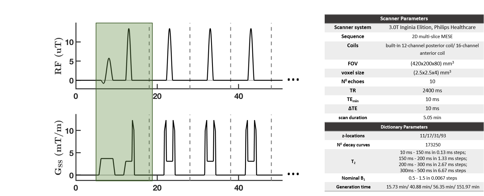
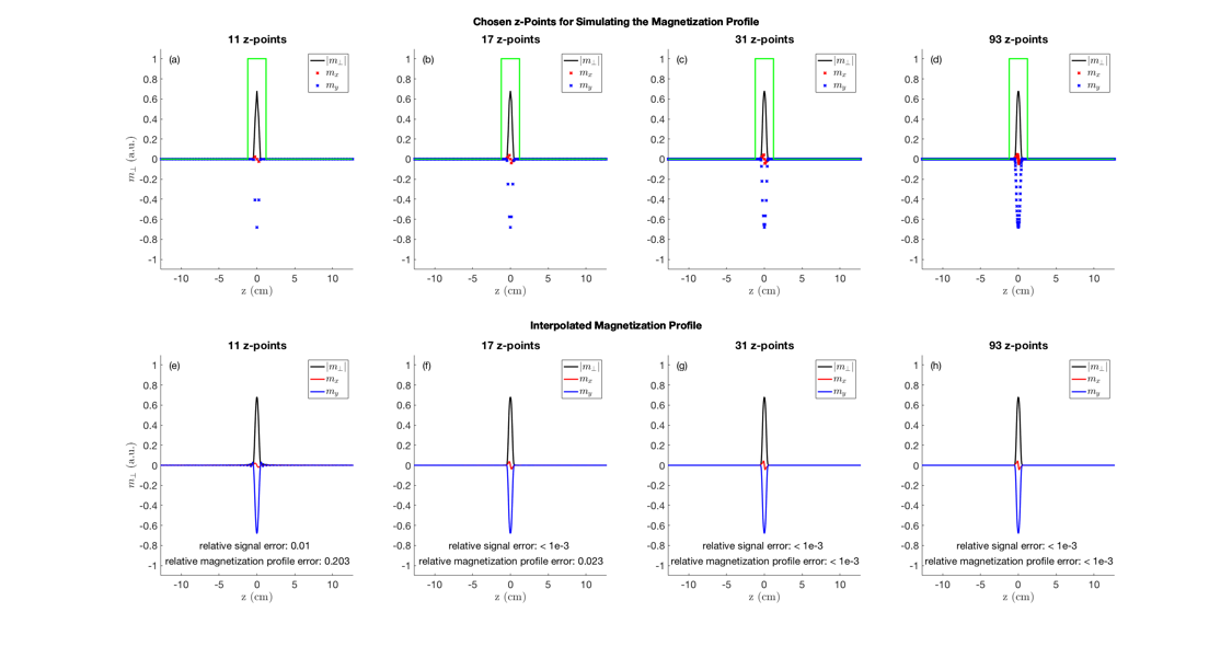
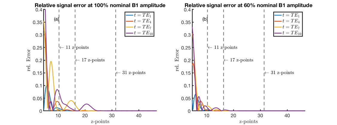
Figure 1 shows the used sequence. To compare the relative error in the magnetization evolution, the magnetization profile was simulated for the first echo for 11, 17, 31 and 93 z-locations over the slab (thickness≈ 2.4cm). An integration over the frequency-encoding-direction was performed (discretization steps: 41). To interpolate the data for comparison, the magnetization profile was transformed into Fourier space, zero-padded and back transformed into real space. The resulting magnetization profile and overall magnetization (= sum over the magnetization profile) was then compared with the reference magnetization profile (at 5001 z-locations over the periodicity interval). To estimate the influence of the spatial sampling density on the magnetization evolution, the relative error of the overall magnetization at four echoes was simulated for different numbers of z-locations for a 60% and 100% nominal B1 amplitude.
Results:
31 and 93 z-locations give the same magnetization profile, whereas fewer z-locations result in profile errors with no influence on the total slice magnetization (17 z-locations). For even less z-locations (11 z-locations) also the signal amplitude changes (Figure 2).
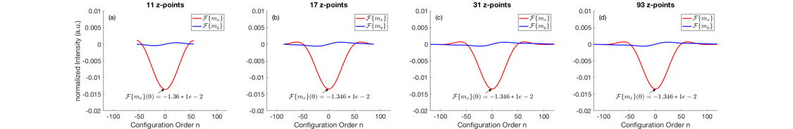
The Fourier transform of the magnetization profiles gives additional insights into the observed effects (Figure 3). Decreasing the amount of z-locations under a critical value (defined by 2N+1 sampling points) causes aliasing in Fourier domain (Figure 3(a)-(b)). However, aliasing at the edges does not influence the 0th configuration component, which is associated with the total slice magnetization. When further reducing the amount of z-locations, aliasing starts affecting the 0th Fourier component which eventually alters the total slice magnetization (Figure 3(a)).
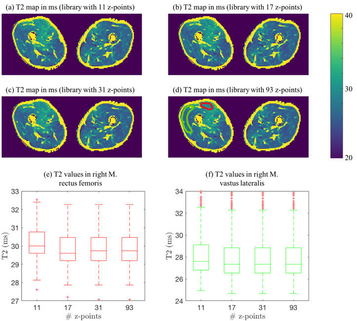
Figure 4 shows that the error in the total slice magnetization is minor for 31 z-locations, whereas it increases for 17 and even more for 11 z-locations. Figure 5 shows in vivo T2 maps post-processed using dictionaries with different z-samplings. Visually, the T2 maps in Figure 5(a)-(d) hardly differ. In the M. rectus femoris and M. vastus lateralis significant differences in the T2 values were obtained with the dictionary using 11 z-locations (p<10-3), no significant differences are observed for higher z samplings. For 31 and 93 z-locations the same T2 values were observed.
Discussion & Conclusion:
The results show that Bloch simulations require considerably less z-locations than used in previous works4,8. To resolve the magnetization profile, more z-locations are needed to include higher frequencies, which describe sharp profile edges. Too few simulated z-locations cause aliasing in Fourier domain, resulting in a wrong slice profile but not affecting the total slice magnetization.
The present work gives educational insights of the connection between the time-domain and slice profile discretization. The results can be applied to speed up dictionary calculations and may be useful in RF-pulse design.
Acknowledgements
The present work was supported by the European Research Council (grant agreement No 677661, ProFatMRI). This work reflects only the authors view and the EU is not responsible for any use that may be made of the information it contains. The authors would also like to acknowledge research support from Philips Healthcare.
References
1. Carlier PG, Marty B, Scheidegger O, et al. Skeletal Muscle Quantitative Nuclear Magnetic Resonance Imaging and Spectroscopy as an Outcome Measure for Clinical Trials. Journal of Neuromuscular Diseases. 2016;3(1):1-28.
2. Carlier PG, Azzabou N, de Sousa PL, et al. Skeletal muscle quantitative nuclear magnetic resonance imaging follow-up of adult Pompe patients. Journal of Inherited Metabolic Disease. 2015;38(3):565-572
3. Mankodi A, Azzabou N, Bulea T, et al. Skeletal muscle water T2 as a biomarker of disease status and exercise effects in patients with Duchenne muscular dystrophy. Neuromuscular Disorders. 2017;27(8):705-714
4. Lebel RM, Wilman AH. Transverse relaxometry with stimulated echo compensation. Magnetic Resonance in Medicine. 2010; 64(4): 1005-1014
5. Marty B, Baudin PY, Reyngoudt H et al. Simultaneous muscle water T2 and fat fraction mapping using transverse relaxometry with stimulated echo compensation. NMR in Biomedicine. 2016;29(4): 431-443
6. Ganter C. Configuration Model. ISMRM 2018. Program #5663
7. Bernstein M, King K, Zhou X. Handbook of MRI Pulse Sequences, 1st Edition. Elsevier. September 7, 2004. ISBN: 9780120928613
8. McPhee KC, Wilman AH. Transverse relaxation and flip angle mapping: Evaluation of simultaneous and independent methods using multiple spin echoes. Magnetic Resonance in Medicine. 2016;77(5): 2057-2065
Figures