Synopsis

Arterial Spin Labeling (ASL) is a non-contrast MR perfusion imaging technique. Pseudo continuous ASL (pCASL) is one of its recomended implementations. The efficiency of pCASL has been shown to be dependent on velocity and magnetic field variations. pCASL was assessed through simulations for the measured velocities in the aorta and including off-resonance effects. Five volunteers were imaged with different average gradient to ratio combinations. The results showed that aorta velocities and off-resonance effects shifted the efficiency towards lower ratios and to a constrained smaller range of gradients. A p-value of 0.04 demonstrated that differences in efficiency were significant across Gave values.

INTRODUCTION

Arterial Spin Labeling (ASL) is a non-contrast MR perfusion imaging technique which uses magnetically labeled arterial blood water as endogenous tracer. According to recommended ASL implementations (1), pseudo-continuous ASL (pCASL) (2-3) is the optimal ASL labeling method in brain. pCASL labelling efficiency has been shown to be dependent on blood velocity and field inhomogeneities near inversion plane location, which may vary across subjects (4-5).

In renal PCASL, off-resonance effects could be exacerbated due to the location of the inversion plane near air-tissue and bone-tissue interfaces. Moreover, aorta is a very pulsatile artery in which moving blood water spins reach high velocities. Therefore, applied radiofrequency (RF) pulses and gradients must be carefully selected in pCASL to optimize efficiency for blood velocities in aorta and to reduce efficiency losses due to off-resonance.

Thus, the goal of this work was to optimize pCASL for its application in renal ASL. This was done through simulations and corroborated by experimental data.

MATERIALS AND METHODS

All participants were scanned in a 3T Skyra system (Siemens, Erlangen, Germany), using an 18-channel body coil, after signing a written informed consent.

Aorta blood flow characterization:

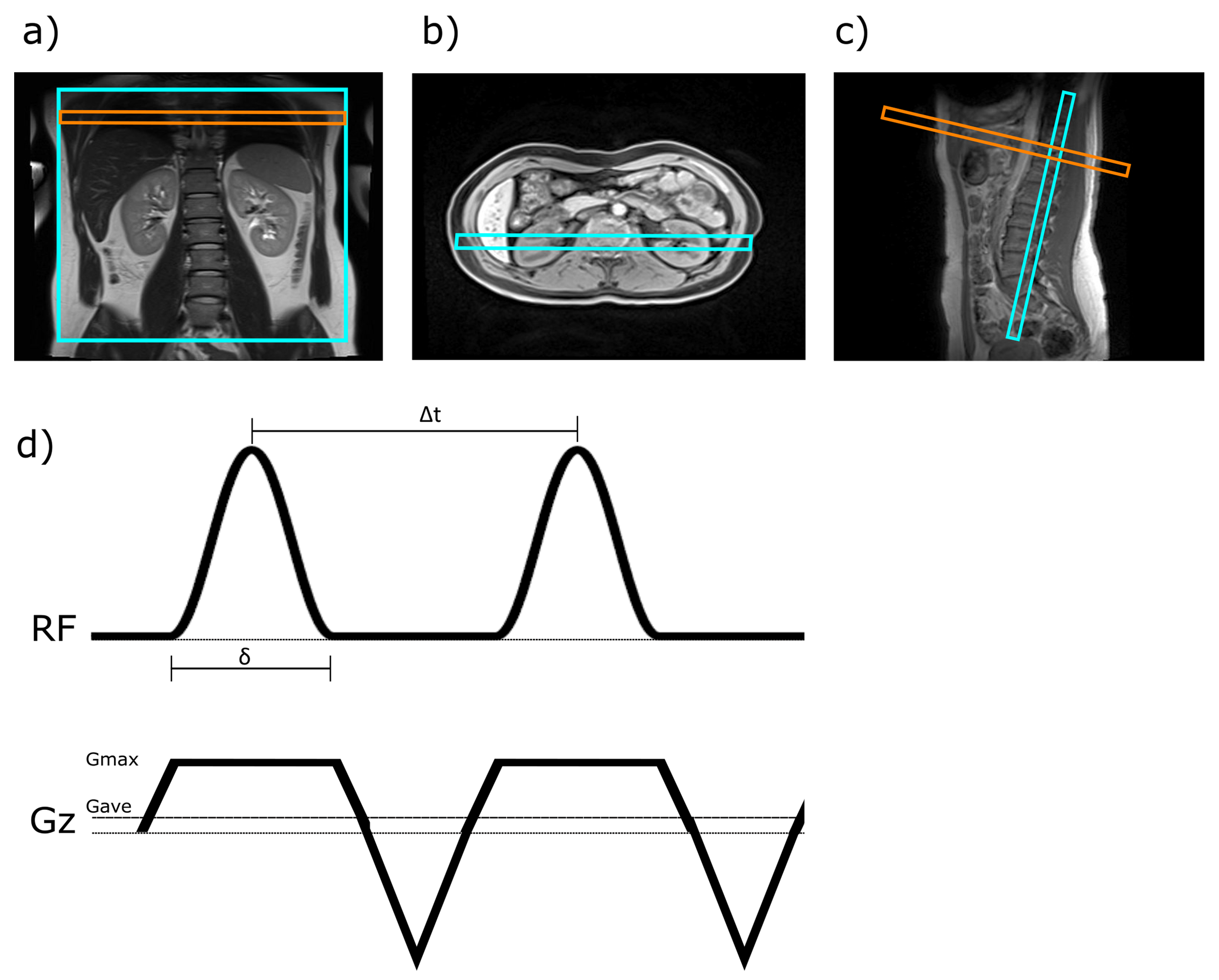
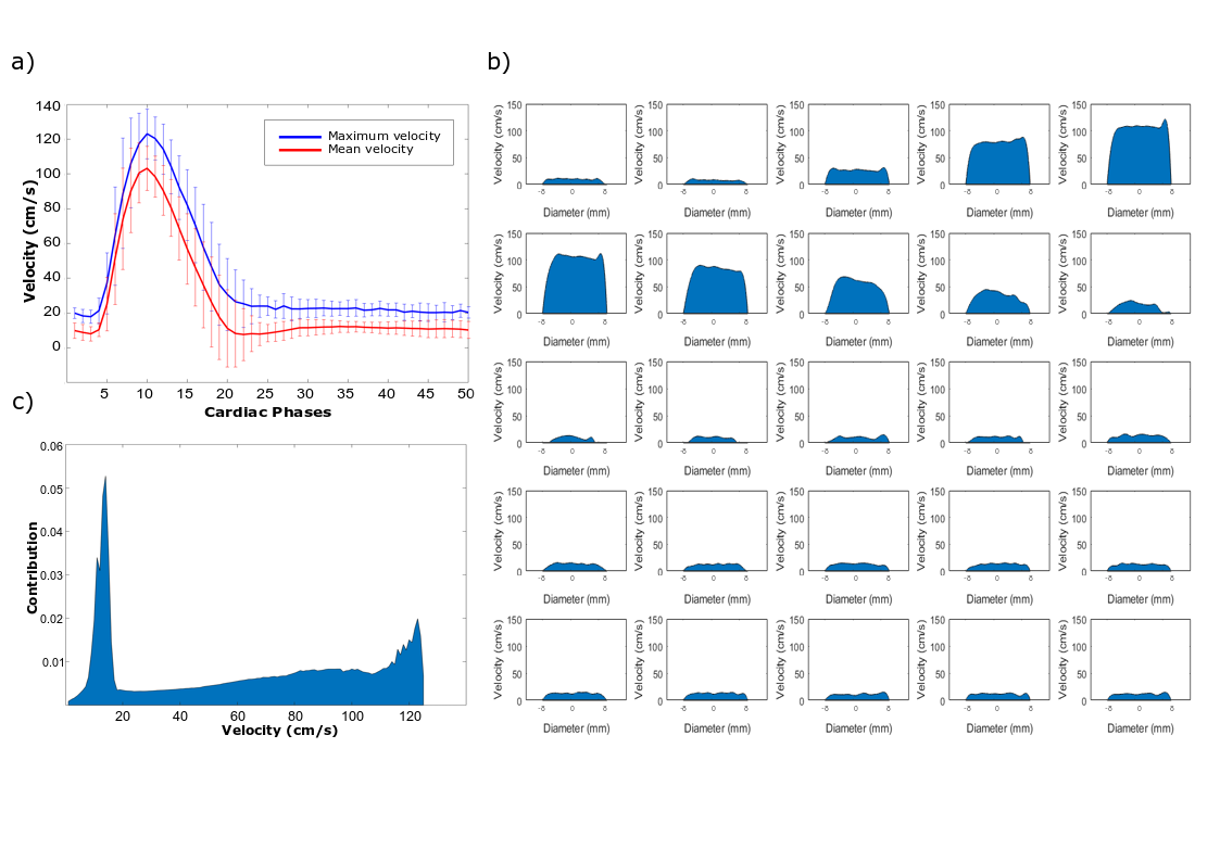
Initially, blood velocity profile was characterized near the pCASL labelling plane location (Fig.1). Eight volunteers (age=29±3 years) were imaged using a cardiac-gated phase-contrast sequence. Velocity curves were averaged among volunteers and contribution of each velocity was calculated for the total duration of the cardiac cycle (Fig.2).

Numerical simulations:

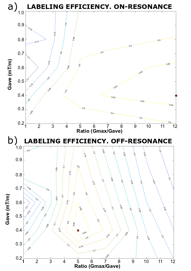
Inversion efficiency was numerically evaluated over a wide range of pCASL parameters. Simulations were based on numerical integration of Bloch equations using an approach previously described (6). Fig.1:c shows labeling pulse sequence. Blood T1 and T2 were 1650ms and 250ms. Average RF-pulse amplitude (B1) was set at 1.6μT, which is a practicable value at 3T. Hann-shaped RF-pulses of 500μs were used followed by 500μs gaps, chosen based on RF duty-cycle limitations in our scanner. Step size was 5μs. Average gradient strengths (Gave) of 0.2-1.0mT/m were evaluated and the ratio of maximum gradient (Gmax) to Gave was varied from 1 to 12. Simulations were performed firstly for on-resonance conditions and subsequently, magnetic field variations were assessed by simulating a range of off-resonance frequencies (0-500Hz). Simulations were implemented in Matlab (Mathworks) running on an Intel® Core™ i3-6100.

Magnetization was evaluated 4cms from the tagging plane and corrected for T1 decay. Efficiency was weighted by the contribution of each velocity (Fig.2:c) and across off-resonance values as proposed in (4).

ASL experiment:

Five subjects participated in this study (age=33±9 years).

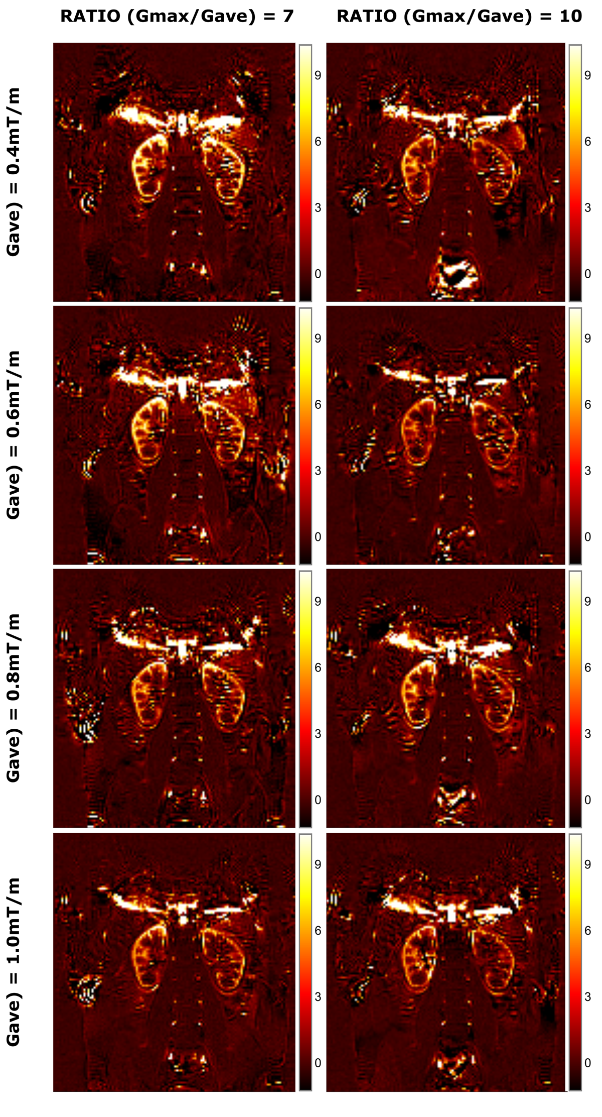
Eight unbalanced pCASL configurations were evaluated, varying across four Gave values (0.4, 0.6, 0.8, 1mT/m) and two ratios (7, 10). Other parameters were according to simulations. Post-labeling delay was 1200ms.

Images were acquired using a bSSFP readout (TR/TE=4500/1.96ms, FOV=400x400mm, FA=50°, matrix=128x128, GRAPPA-2). Presaturation pulses were applied at the beginning of each TR. Labelling plane was oriented perpendicularly to the descending aorta and 10cm above the center of the kidneys (Fig.1:a-c). Respiratory triggering was used to acquire 25 pairs of control-label images, using a threshold of 90% of the maximum inspiration peak so as to acquire the image in expiration phase.

Images were registered using Advance Normalization Tools (ANTS). Mean ASL signal was computed for each pair, and outliers (considered as being more than 2 SD away from the global mean) were discarded. Total perfusion signal, calculated as the mean signal of the corrected pairs, was measured across a manually-defined bilateral ROI in the kidneys. A two-way analysis of variance (ANOVA) was calculated to examine the relationship between perfusion signal and gradient parameters.

RESULTS

Aorta blood flow characterization: Velocity profiles are shown in Fig.2:c. The range of velocities in aorta varied from 17cm/s to 123cm/s.

Numerical simulations: For on-resonance conditions, efficiencies are over 0.9 for a large range of Gave (0.3-0.7) and ratios over 5. In presence of off-resonance effects, the higher efficiencies are shifted towards lower ratios and constrained to a smaller range of Gave (Fig.3).

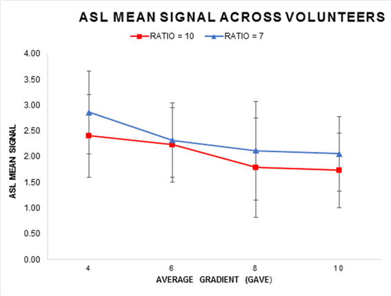
ASL experiment: Fig.4:a-g shows renal perfusion images acquired in one volunteer across all tested Gave-Ratio configurations. Fig. 5 shows the mean perfusion signal across the group. The results were in agreement with the numerical simulations: higher efficiencies were found when using lower Gave gradients and lower ratios. A p-value of 0.04 demonstrated that differences in efficiency were significant across Gave values.

CONCLUSION

Acknowledgements

References

1. Alsop DC, Detre JA, Golay X, Günther M, Hendrikse J, Hernandez-Garcia L, et al. Recommended implementation of arterial spin-labeled Perfusion mri for clinical applications: A consensus of the ISMRM Perfusion Study group and the European consortium for ASL in dementia. Magn Reson Med. 2015;73(1):102–16.

2. Dai W, Garcia D, De Bazelaire C, Alsop DC. Continuous flow-driven inversion for arterial spin labeling using pulsed radio frequency and gradient fields. Magn Reson Med. 2008;

3. Wu WC, Fernández-Seara M, Detre JA, Wehrli FW, Wang J. A theoretical and experimental investigation of the tagging efficiency of pseudocontinuous arterial spin labeling. Magn Reson Med. 2007;58(5):1020–7.

4. Zhao L, Vidorreta M, Soman S, Detre JA, Alsop DC. Improving the robustness of pseudo-continuous arterial spin labeling to off-resonance and pulsatile flow velocity. Magn Reson Med. 2017;78(4):1342–51.

5. Jahanian H, Noll DC, Hernandez-Garcia L. B 0 field inhomogeneity considerations in pseudo-continuous arterial spin labeling (pCASL): Effects on tagging efficiency and correction strategy. NMR Biomed. 2011;24(10):1202–9.

6. Maccotta L, Detre J a, Alsop DC. The efficiency of adiabatic inversion for perfusion imaging by arterial spin labeling. NMR Biomed. 1997;10(4–5):216–21.