4937
Functional quantitative susceptibility mapping (fQSM) during auditory stimulation1Imago7 and IRCCS Stella Maris, Pisa, Italy, 2IMT School for Advanced Studies, Lucca, Italy, 3University of Pisa, Pisa, Italy
Synopsis
Functional Quantitative Susceptibility Mapping (fQSM) has two very appealing and promising features: it is a quantitative way of mapping brain function and it is considerably less affected by the non-local effects typical of the Blood Oxygenation Level-Dependent (BOLD) signal. Here, the response of the auditory cortex to the presentation of relatively short acoustic stimuli has been studied. The majority of voxels with positive BOLD responses exhibited negative fQSM responses, while some other voxels exhibited positive fQSM repsonses, which might reflect different interplays among changes in fractional oxygen saturation, cerebral blood flow and volume.
Introduction
Quantitative Susceptibility Mapping (QSM) is a novel technique1-4 that uses the information of signal phase to remove, by deconvolution, the non-local dipole effects in the data5-7, to achieve quantitative maps of the local changes in magnetic susceptibility. Only a small body of literature has applied QSM to functional studies (fQSM). These studies investigated the brain responses to visual8-12, somatosensory9 and motor8,9,13 tasks, as well as in resting state10, and they highlighted the potential of fQSM. However, to date this new approach is still largely unexplored and several aspects are under debate. Our aim was to increase our understanding of fQSM brain responses. The target region of our study was the auditory cortex, which has not yet been explored in the published literature on fQSM.Methods
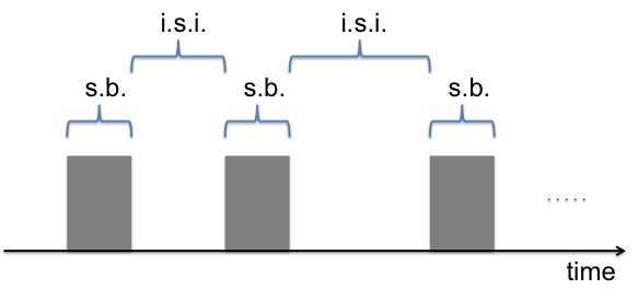
The data of four healthy subjects were acquired with a GE MR950 7T scanner. For each subject, the acquisition protocol included two 2D gradient-recalled Echo Planar Imaging (EPI) sequences with TR=2.5s, TE=21.3ms, and isotropic voxels of size 1.8×1.8×1.8mm3. Both the magnitude and the phase of the data were saved. During scanning, MRI-compatible earbuds delivered acoustic stimuli to the subject according to the paradigm shown in Figure 1.
Each individual volume of the phase timeseries underwent a well-established pre-processing pipeline that included phase unwrapping14 and background phase removal15. Quantitative values of magnetic susceptibility χ (fQSM) were obtained from the phase data16 by using the iLSQR algorithm7. The magnitude images were coregistered to the first time frame of the first acquisition of each subject17 and the transformation matrices were applied also to the timeseries of fQSM data. Slow temporal drifts in the timeseries were removed by a high-pass filter (retaining the DC component) with a cutoff frequency of 0.02Hz. To avoid any assumption on the shape of fQSM responses, the mean responses to the stimuli were computed by using a data-driven approach based on signal deconvolution on each voxel18-20 with goodness-of-deconvolution evaluated in terms of r2, with 0≤r2≤119. Statistics (P-values) for the r2 values were obtained by using a permutation analysis method: by taking the r2 value that ranked as the 99% highest value in the chance distribution, a cutoff r2 value to select volxels with P<0.01 was identified19. A value of r2=0.1 was obtained for both BOLD and fQSM. Regions of interest (ROIs) were manually drawn in the BOLD maps thresholded at P<0.01, around the clusters of active voxels in the auditory cortex21. For each voxel that exhibited statistically significant activations in both BOLD and fQSM, the following items describing the stimulus responses were considered: r2, timecourse of the stimulus response, mean of the voxel timecourse, peak of the response. The relationships among these items were assessed with scatter plots, linear fits and Pearson’s coefficients of linear correlation.
Results
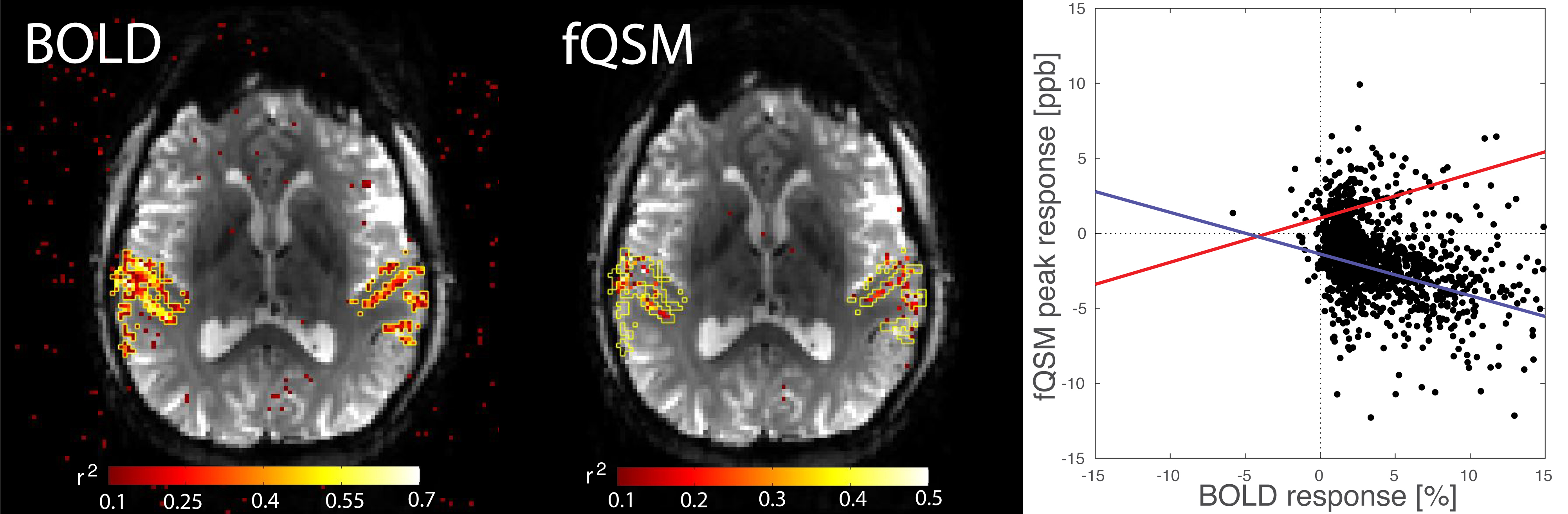
Figure 2 shows that activated voxels in fQSM were fewer than in BOLD fMRI (17% on average across subjects, for the same threshold of r2>0.1). The 82% of activated voxels had responses with opposite sign in fQSM with respect to BOLD, while the remaining voxels exhibited BOLD and fQSM responses of the same sign.
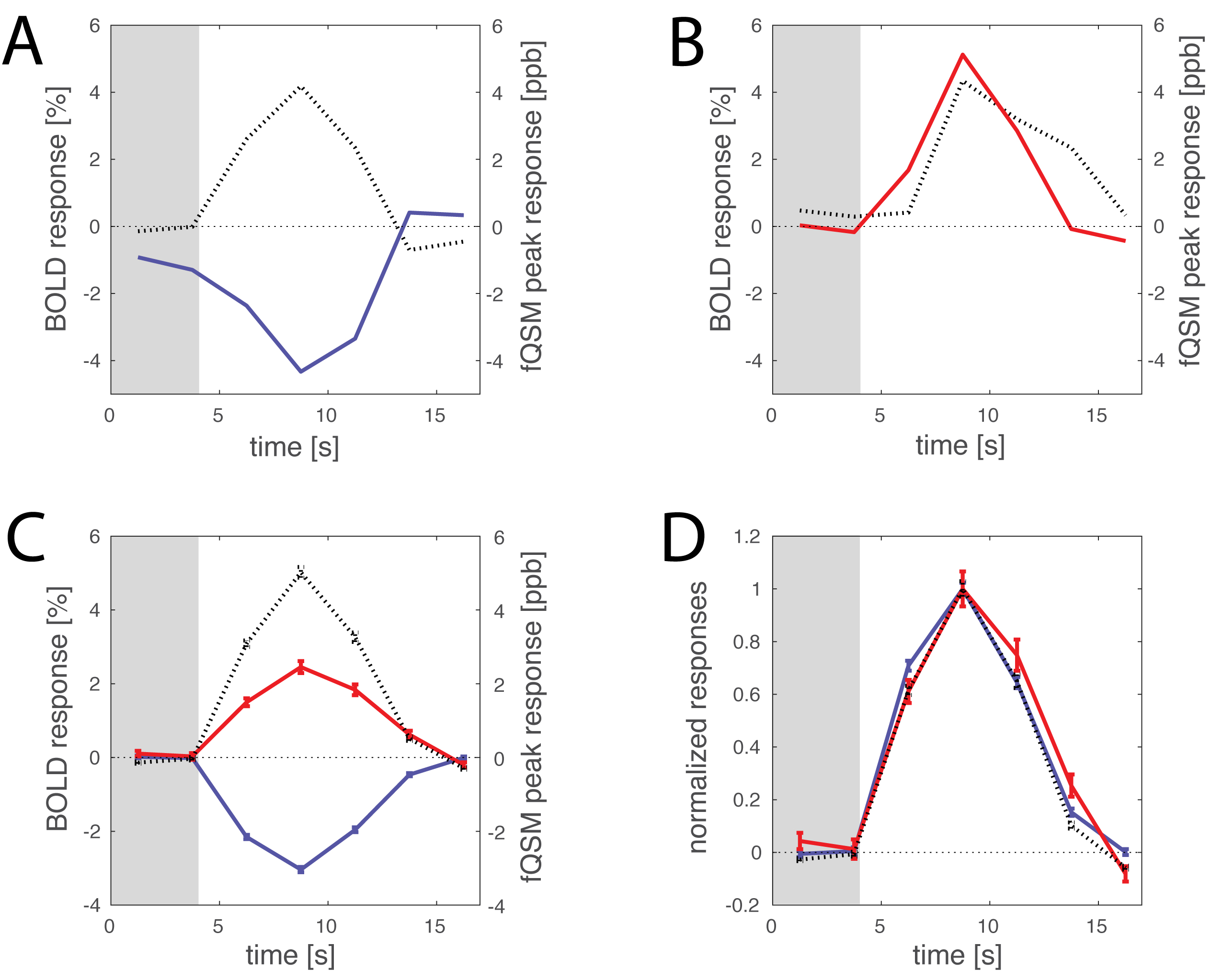
The shapes of the fQSM responses were very similar to that of the average BOLD response, with peak values that occurred about 6s after the end of the stimulation event (Figure 3).
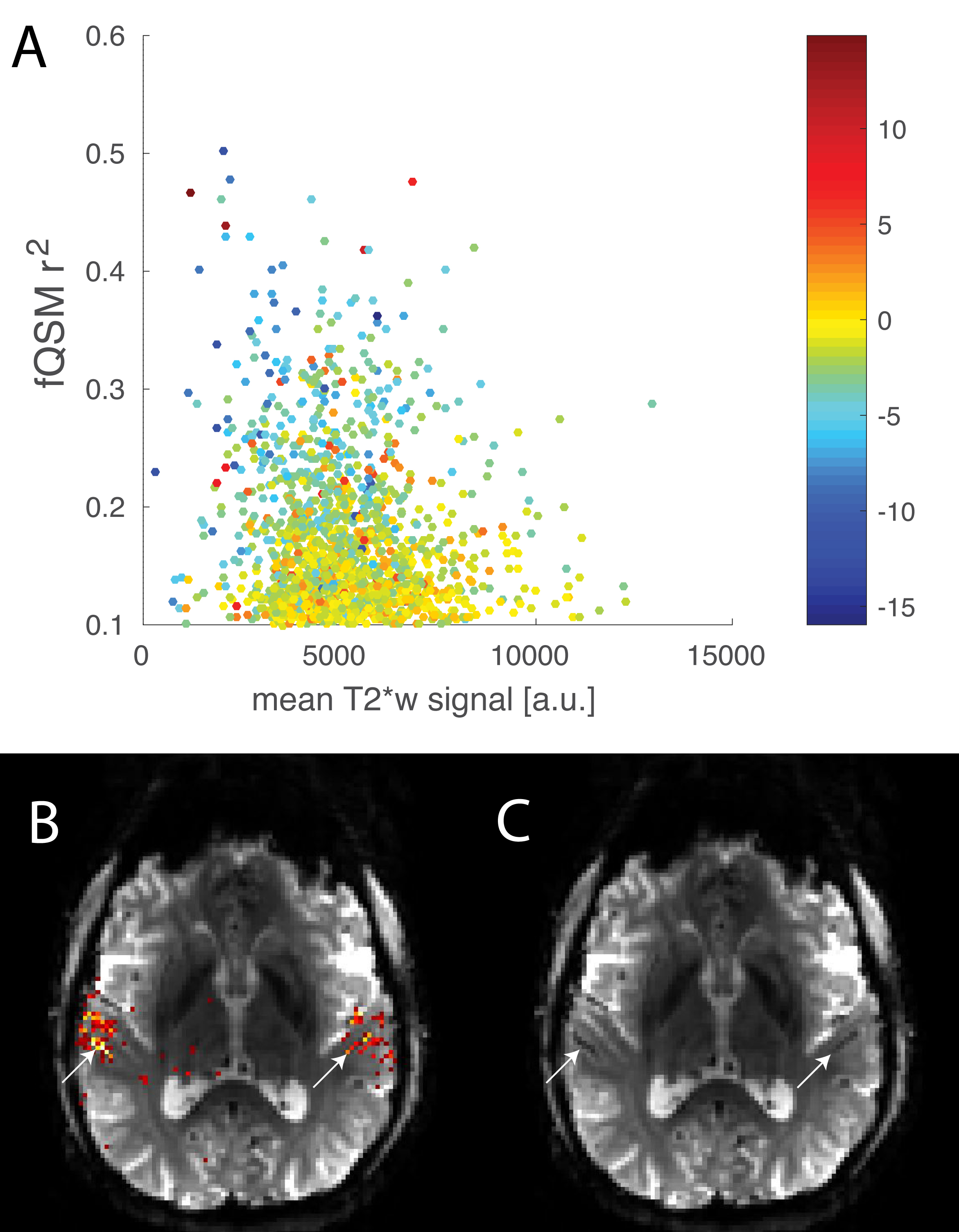
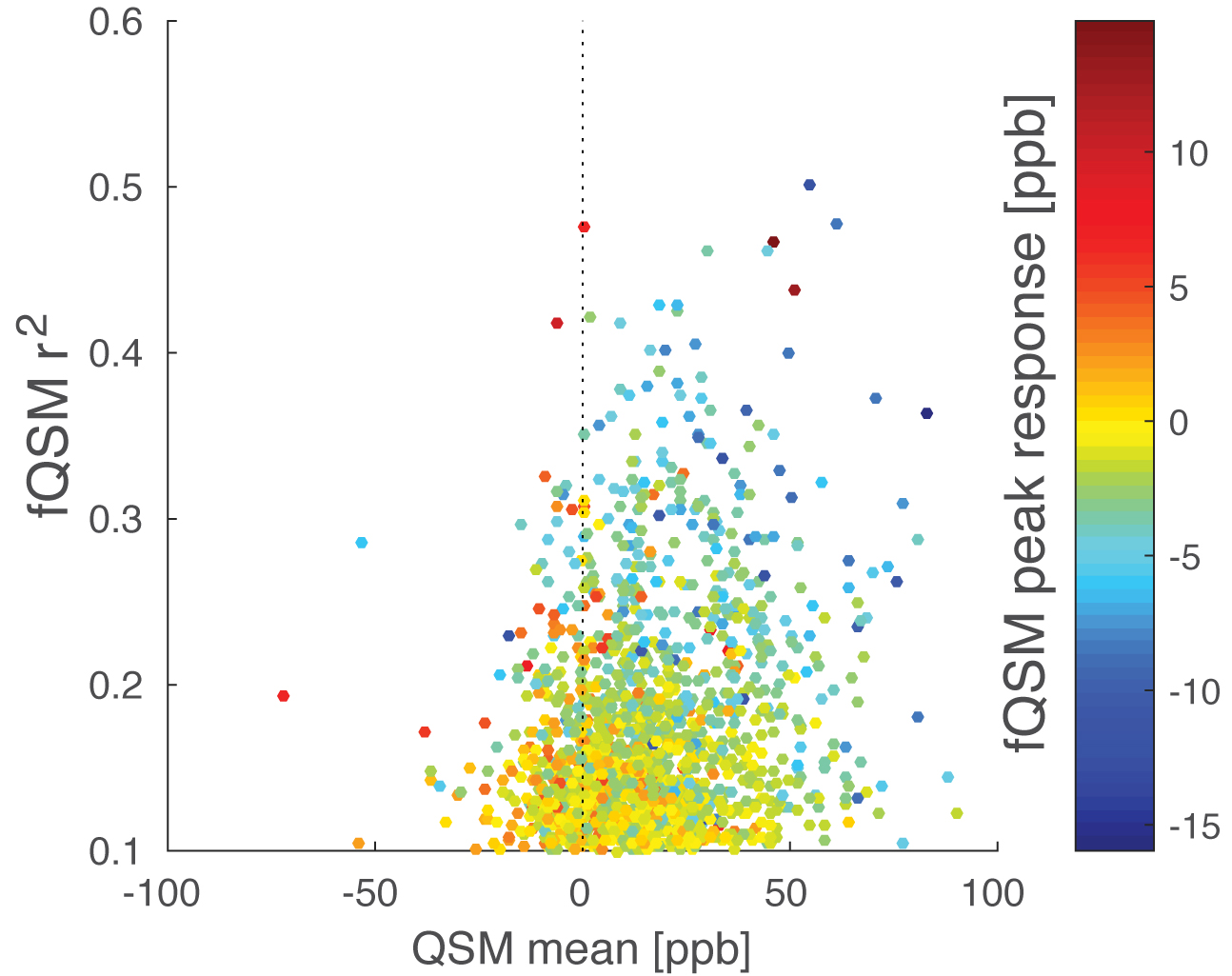
Figure 4 shows the relationship among fQSM r2 values, the mean T2*-weighted signal of the EPI images, and the fQSM peak responses. The highest r2 values in fQSM correspond to T2*-hypointense voxels which represent veins, where negative fQSM responses beyond -10ppb occur. However, high fQSM r2 values (r2>0.3) were observed also in non-vein voxels that had, for the most part, small negative fQSM responses -5<χ<0 ppb (green and yellow dots in Figures 4A and 5) and moderately positive (0<χ<50ppb) QSM mean values (Figure 5), typical of cortical gray matter9,22,23, as confirmed by retrospective manual inspection of the data. The majority of voxels with positive fQSM responses had moderately negative QSM mean values (Figure 5, red dots) that are typically associated to white matter24.
Discussion
A current matter of debate is the interpretation of positive fQSM responses. It cannot be excluded that they originate from incorrect phase-dipole deconvolution9,11 and/or defective measures depending on tissue orientation25,26, however this type of confounds should not affect the cortex27. Positive fQSM responses might capture, at least to some extent, variations in the interplay among changes in fractional oxygen saturation, cerebral blood flow and volume8-11. Future studies should aim to verify this hypothesis.Acknowledgements
No acknowledgement found.References
1. Wang, Y. & Liu, T. Quantitative susceptibility mapping (QSM): Decoding MRI data for a tissue magnetic biomarker. Magn. Reson. Med. 73, 82–101 (2015).
2. Haacke, E. M. et al. Quantitative susceptibility mapping: current status and future directions. Magn Reson Imaging 33, 1–25 (2015).
3. Deistung, A., Schweser, F. & Reichenbach, J. R. Overview of quantitative susceptibility mapping. NMR in Biomedicine (2016). doi:10.1002/nbm.3569
4. Liu, C., Li, W., Tong, K. A., Yeom, K. W. & Kuzminski, S. Susceptibility-weighted imaging and quantitative susceptibility mapping in the brain. Journal of Magnetic Resonance Imaging 42, 23–41 (2015).
5. de Rochefort, L. et al. Quantitative susceptibility map reconstruction from MR phase data using bayesian regularization: Validation and application to brain imaging. Magn. Reson. Med. 63, 194–206 (2010).
6. Liu, T. et al. Morphology enabled dipole inversion (MEDI) from a single‐angle acquisition: Comparison with COSMOS in human brain imaging. Magn. Reson. Med. 66, 777–783 (2011).
7. Li, W. et al. A method for estimating and removing streaking artifacts in quantitative susceptibility mapping. NeuroImage 108, 111–122 (2015).
8. Chen, Z., Liu, J. & Calhoun, V. D. Susceptibility-based functional brain mapping by 3D deconvolution of an MR-phase activation map. Journal of Neuroscience Methods 216, 33–42 (2013).
9. Balla, D. Z. et al. Functional quantitative susceptibility mapping (fQSM). NeuroImage 100, 112–124 (2014).
10. Bianciardi, M., van Gelderen, P. & Duyn, J. H. Investigation of BOLD fMRI resonance frequency shifts and quantitative susceptibility changes at 7 T. Hum. Brain Mapp. 35, 2191–2205 (2014).
11. Özbay, P. S. et al. Probing neuronal activation by functional quantitative susceptibility mapping under a visual paradigm: A group level comparison with BOLD fMRI and PET. NeuroImage 137, 52–60 (2016).
12. Sun, H., Seres, P. & Wilman, A. H. Structural and functional quantitative susceptibility mapping from standard fMRI studies. NMR in Biomedicine 30, e3619 (2017).
13. Chen, Z., Robinson, J., Caprihan, A. & Calhoun, V. High-resolution human brain functional χ mapping reveals focal and bidirectional BOLD responses. Biomed. Phys. Eng. Express 3, 015027 (2017).
14. Schofield, M. A. & Zhu, Y. Fast phase unwrapping algorithm for interferometric applications. Opt Lett 28, 1194–1196 (2003).
15. Schweser, F., Deistung, A., Lehr, B. W. & Reichenbach, J. R. Quantitative imaging of intrinsic magnetic tissue properties using MRI signal phase: An approach to in vivo brain iron metabolism? NeuroImage 54, 2789–2807 (2011).
16. Shmueli, K. et al. Magnetic susceptibility mapping of brain tissue in vivo using MRI phase data. Magn. Reson. Med. 62, 1510–1522 (2009).
17. Jenkinson, M., Bannister, P., Brady, M. & Smith, S. Improved Optimization for the Robust and Accurate Linear Registration and Motion Correction of Brain Images. NeuroImage 17, 825–841 (2002).
18. Dale, A. M. Optimal experimental design for event-related fMRI. Hum. Brain Mapp. 8, 109–114 (1999).
19. Gardner, J. L. et al. Contrast Adaptation and Representation in Human Early Visual Cortex. Neuron 47, 607–620 (2005).
20. Costagli, M. et al. Functional Signalers of Changes in Visual Stimuli: Cortical Responses to Increments and Decrements in Motion Coherence. Cerebral Cortex 24, 110–118 (2014).
21. Humphries, C., Liebenthal, E. & Binder, J. R. Tonotopic organization of human auditory cortex. NeuroImage 50, 1202–1211 (2010).
22. Barbosa, J. H. O. et al. Quantifying brain iron deposition in patients with Parkinson's disease using quantitative susceptibility mapping, R2 and R2. Magn Reson Imaging 33, 559–565 (2015).
23. Costagli, M. et al. Magnetic susceptibility in the deep layers of the primary motor cortex in Amyotrophic Lateral Sclerosis. Neuroimage Clin 12, 965–969 (2016).
24. Lim, I. A. L. et al. Human brain atlas for automated region of interest selection in quantitative susceptibility mapping: Application to determine iron content in deep gray matter structures. NeuroImage 82, 449–469 (2013).
25. Denk, C., Torres, E. H., MacKay, A. & Rauscher, A. The influence of white matter fibre orientation on MR signal phase and decay. NMR in Biomedicine 24, 246–252 (2011).
26. Wharton, S. & Bowtell, R. Effects of white matter microstructure on phase and susceptibility maps. Magn. Reson. Med. 73, 1258–1269 (2015).
27. Lancione, M., Tosetti, M., Donatelli, G., Cosottini, M. & Costagli, M. The impact of white matter fiber orientation in single-acquisition quantitative susceptibility mapping. NMR in Biomedicine 30, e3798 (2017).
Figures