4931
SHARQnet - Sophisticated Harmonic Artifact Reduction in Quantitative Susceptibility Mapping using a Deep Convolutional Neural Network1Department of Health Science and Technology, Aalborg University, Aalborg East, Denmark, 2Centre for Advanced Imaging, The University of Queensland, Brisbane, Australia, 3Siemens Healthcare Pty Ltd, Brisbane, Australia, 4Department of Neurology, Medical University of Graz, Graz, Austria
Synopsis
We propose a fully convolutional neural network for background field removal in MR phase images for Quantitative Susceptibility Mapping. Our proposed method, SHARQnet, learns to solve the background field problem from theoretical simulations of background field distributions, and the results are compared to current state-of-the-art methods like SHARP, V-SHARP, and RESHARP.
INTRODUCTION
Quantitative susceptibility mapping (QSM) extracts magnetic susceptibility from MR signal phase and has the potential to give further insight into neurodegenerative diseases1–3. Background field removal is a fundamental step in the QSM processing pipeline with the goal to remove contributions of the magnetic field from outside the region of interest. The inverse problem relating the measured field perturbation to the underlying magnetic susceptibility distribution can then be solved to provide the final quantitative susceptibility map. Existing background field removal techniques rely on a variety of assumptions, like no or limited low-frequency contents4, the absence of sources close to the boundary2,5, no harmonic internal and boundary fields in boundary regions6,7, or the minimization of an objective function involving a specific error norm8–10. The performance of the existing methods is also dependent on the optimization of regularization parameters4.
Deep learning has been shown to be a powerful method for solving the field-to-source inversion problems of QSM without the use of regularization parameters during prediction11,12 by learning the forward field solution and efficiently solving the inverse problem. We propose a new algorithm to remove the background field from GRE MR phase images based on simulations of realistic field configurations and show that we can solve the problem in a very efficient way.
METHODS
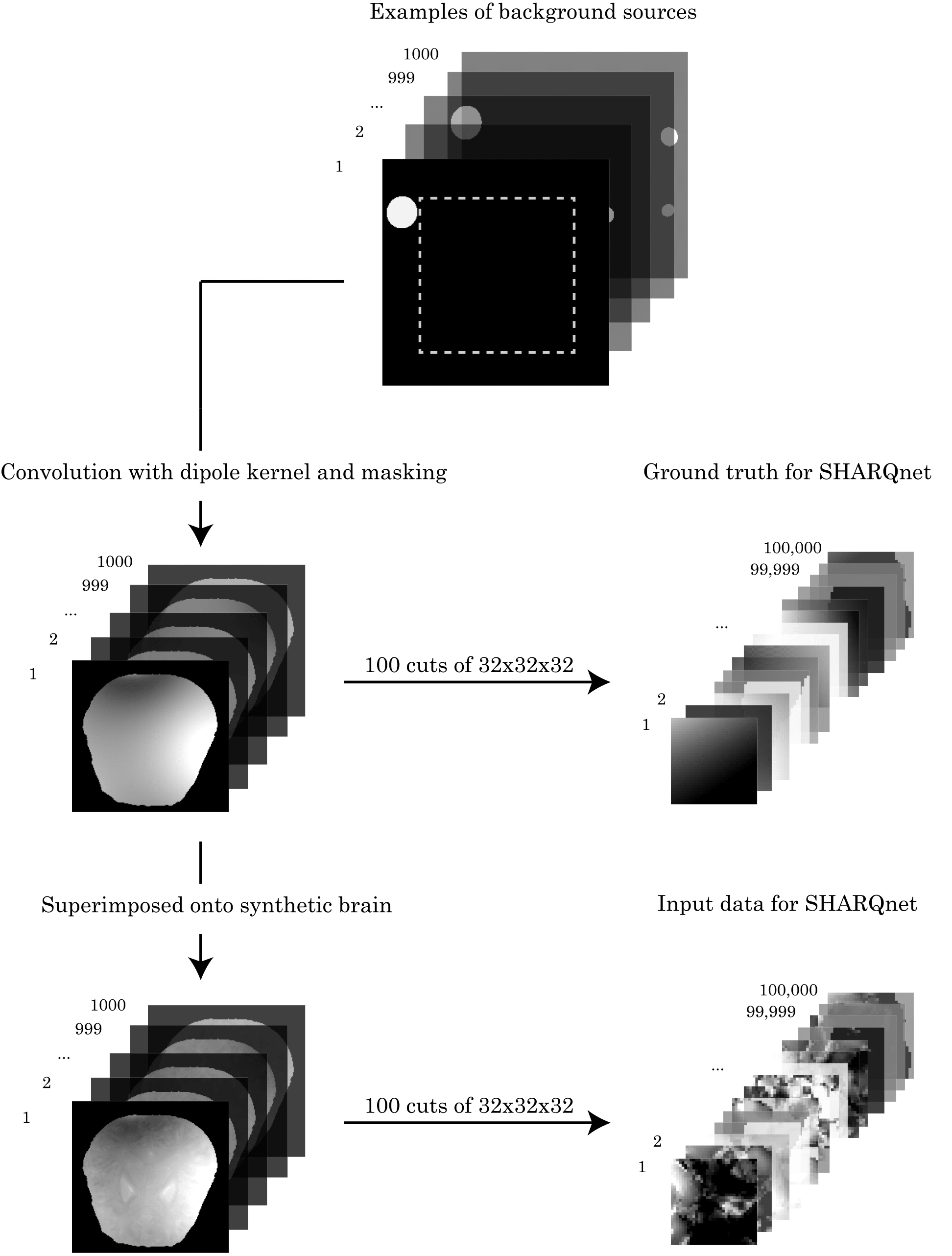
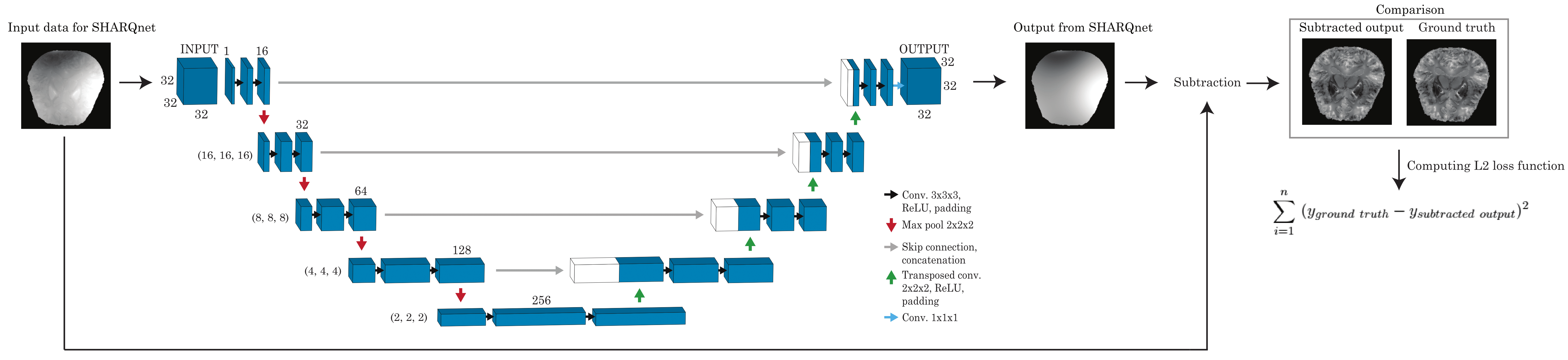
The fully convolutional neural network following a modified U-Net architecture (Figure 1) was implemented using Tensorflow v.1.6 in Python 3.6. The network was trained with 100,000 simulated images with the size of 32x32x32, batch size of 50, and a dropout of 0.15 for 12 hours on NVIDIA Tesla K80(C) GPUs.
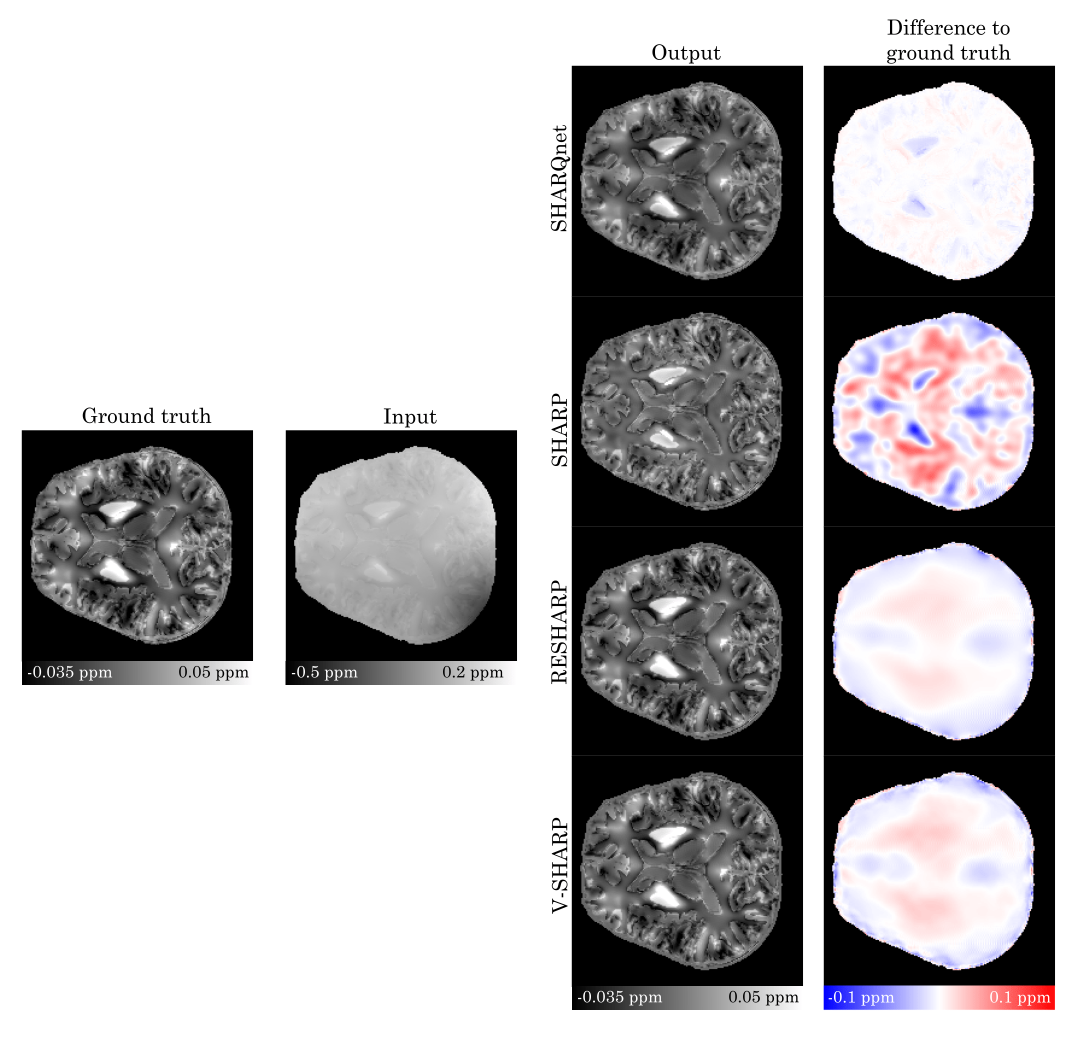
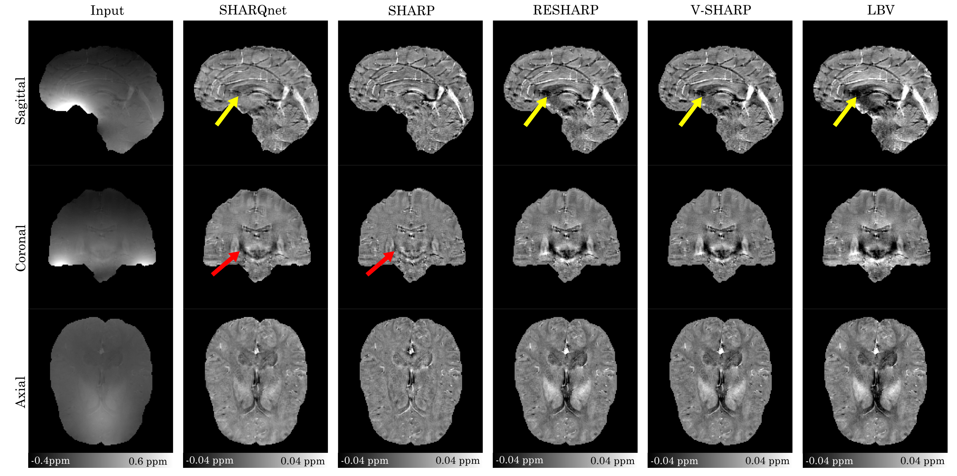
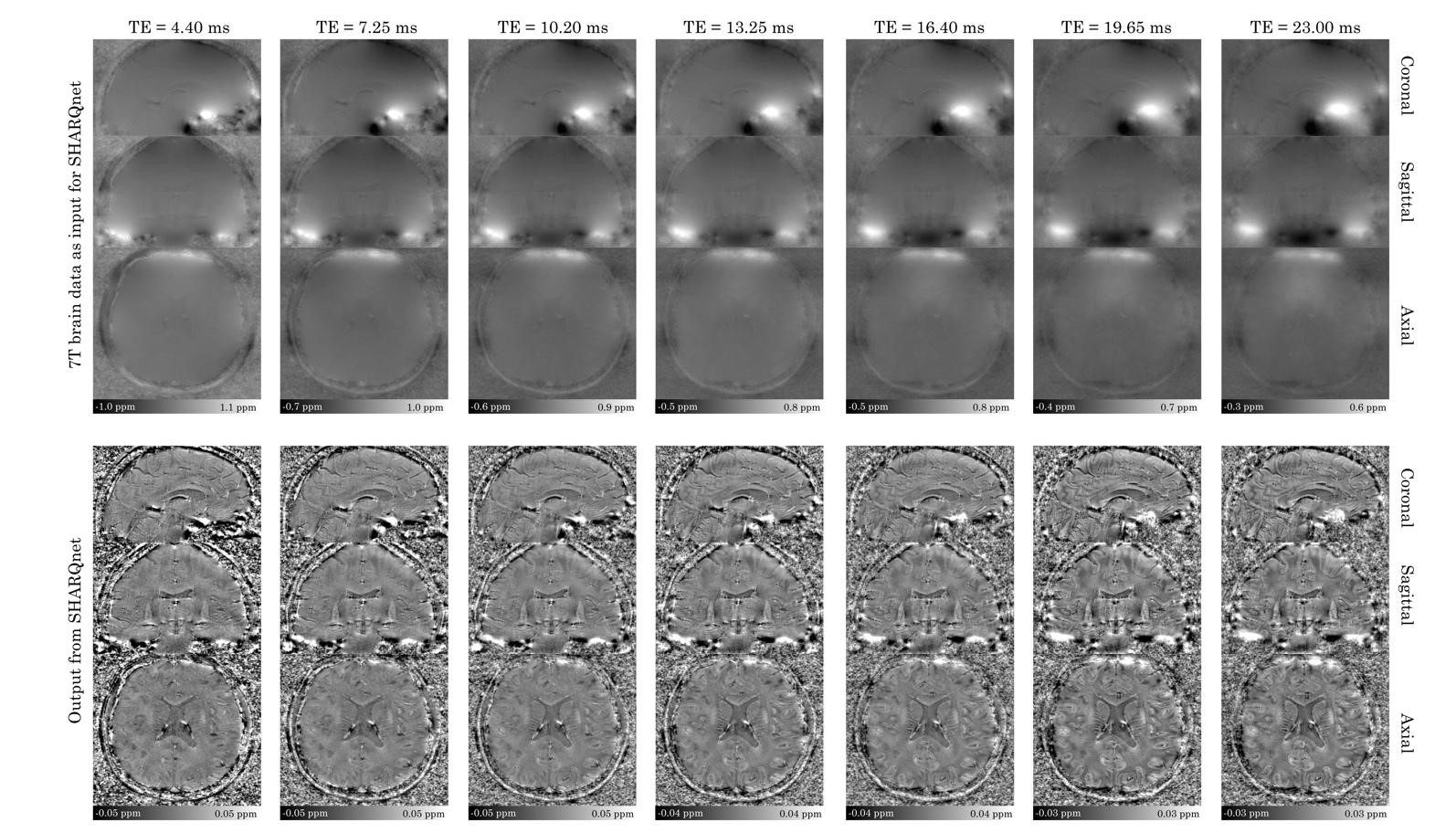
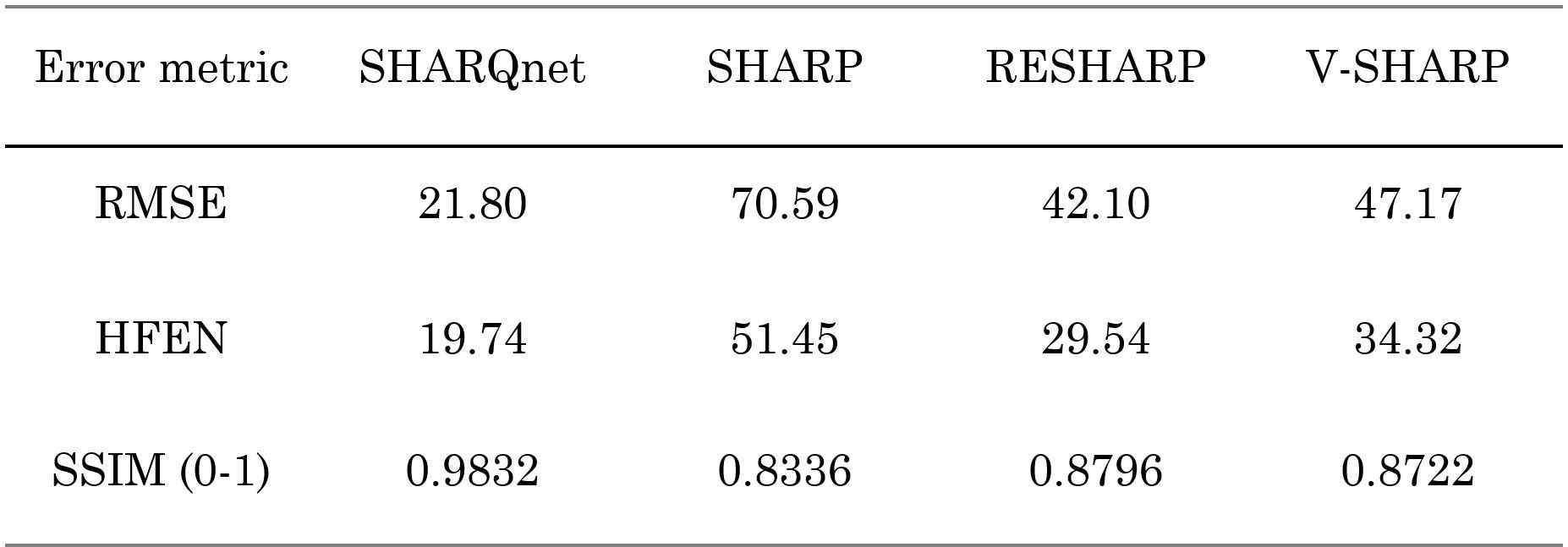
External sources generating the background field were simulated as ellipsoids and placed around a synthetic brain simulation with a susceptibility of 100 parts per million (ppm) relative to water. To increase variance within the training images, the ellipsoids were augmented by randomly varying the number (2-3), the scale, the orientation, and the susceptibility value (±10%). The external sources were convolved with the unit dipole kernel to generate the background fields and superimposed onto a 192x192x192 synthetic brain included in the MEDI toolbox13 serving as input to the network. The simulated background field was used as a target for the network. The network training minimised the error by computing the residual squared error between the predicted background field subtracted from the input and the underlying susceptibility distribution. With this procedure, the network was forced to learn only the background field to ensure not to overfit to structures in the underlying susceptibility distribution of interest. The network was tested on synthetic brain simulations and real-world data from the 2016 QSM reconstruction challenge14. SHARQnet was also tested on a real-world 7T dataset where the skull and surrounding background had not been removed to illustrate the robustness of the newly proposed algorithm. Evaluation of the result of SHARQnet was based on the following error metrics; root-mean-square error (RMSE), high-frequency error norm (HFEN), structural similarity index (SSIM). Additionally, the result was compared to existing methods for background field removal; SHARP2, RESHARP10, and V-SHARP5.
RESULTS/DISCUSSION
SHARQnet’s performance on simulated data produced excellent results (Figure 3) with lower error metrics compared to established methods (Table 1). SHARQnet’s performance on the 2016 QSM reconstruction challenge showed qualitatively very similar results when comparing it to the other existing algorithms (Figure 4). The results show that SHARQnet removes residual background fields better than RESHARP, V-SHARP, and LBV in the center of the brain (See yellow arrows in Figure 4), but at the same time preserves anatomical details better than SHARP (See red arrows in Figure 4). In addition, the test on a high-resolution 7T dataset showed that SHARQnet generalizes to ultra-high-field background field artifacts and may even be used without a brain mask, possibly reducing problems with regard to extracting a brain mask required by established methods (Figure 5).CONCLUSION
We demonstrated that our deep learning–based algorithm produced high quality results with lower error metrics compared to established methods and is a promising solution to the background-field removal problem in QSM with the potential for fast, accurate background field removals that do not require masking.Acknowledgements
This study was supported by the facilities of the National Imaging Facility at the Centre for Advanced Imaging, the University of Queensland, as well as resources and services from the National Computer Infrastructure (NCI), supported by the Australian Government. The four first-mentioned authors acknowledge financial support from the following private organisations: the Obel Family Foundation, the Knud Højgaard Foundation, the Augustinus Foundation, the Oticon Foundation, Otto Mønsted’s Foundation, the Henry and Mary Skov's Foundation, Viet-Jacobsen Foundation, Torben og Alice Frimodt’s Foundation, Aalborg Stiftstidende Foundation, Dansk Tennis Foundation, Marie and M.B. Richters Foundation, Julie Damms Foundation, the Roblon Foundation, Vanggaard Foundation, William and Hugo Evers Foundation, the Frimodt-Heineke Foundation, Statsautoriseret Revisor Oluf Christian Olsen and Hustru Julie Rasmine Olsens Foundation, and Reinholdt W. Jorck og Hustrus Foundation.References
1. Reichenbach JR, Schweser F, Serres B, Deistung A. Quantitative Susceptibility Mapping: Concepts and Applications. Clin Neuroradiol. 2015;25:225–30.
2. Schweser F, Deistung A, Lehr BW, Reichenbach JR. Quantitative imaging of intrinsic magnetic tissue properties using MRI signal phase: An approach to in vivo brain iron metabolism? Neuroimage. 2011;54(4):2789–807. Available from: http://dx.doi.org/10.1016/j.neuroimage.2010.10.070
3. Barbosa JHO, Santos AC, Tumas V, Liu M, Zheng W, Haacke EM, et al. Quantifying brain iron deposition in patients with Parkinson’s disease using quantitative susceptibility mapping, R2 and R2*. Magn Reson Imaging. 2015;33(5):559–65. Available from: http://dx.doi.org/10.1016/j.mri.2015.02.021
4. Schweser F, Robinson SD, de Rochefort L, Li W, Bredies K. An illustrated comparison of processing methods for phase MRI and QSM: removal of background field contributions from sources outside the region of interest. NMR Biomed. 2017;30(4).
5. Wu B, Li W, Guidon A, Liu C. Whole brain susceptibility mapping using compressed sensing. Magn Reson Med. 2012;67(1):137–47.
6. Zhou D, Liu T, Spincemaille P, Wang Y. Background field removal by solving the Laplacian boundary value problem. NMR Biomed. 2014;27(3):312–9.
7. Wen Y, Zhou D, Liu T, Spincemaille P, Wang Y. An Iterative Spherical Mean Value (iSMV) Method for Background Field Removal in MRI. Magn Reson Med. 2014;72(4):1065–71.
8. Liu T, Khalidov I, de Rochefort L, Spincemaille P, Liu J, Tsiouris AJ, et al. A novel background field removal method for MRI using projection onto dipole fields (PDF). NMR Biomed. 2011;24(9):1129–36.
9. Li W, Avram A V., Wu B, Xiao X, Liu C. Integrated Laplacian-based phase unwrapping and background phase removal for quantitative susceptibility mapping. NMR Biomed. 2014;27(2):219–27.
10. Sun H, Wilman AH. Background field removal using spherical mean value filtering and Tikhonov regularization. Magn Reson Med. 2014;71(3):1151–7.
11. Rasmussen KGB, Kristensen MJ, Blendal RG, Ostergaard LR, Plocharski M, O’Brien K, et al. DeepQSM - Using Deep Learning to Solve the Dipole Inversion for MRI Susceptibility Mapping. bioRxiv. 2018; Available from: https://www.biorxiv.org/content/early/2018/03/07/278036
12. Yoon J, Gong E, Chatnuntawech I, Bilgic B, Lee J, Jung W, et al. Quantitative susceptibility mapping using deep neural network: QSMnet. Neuroimage. 2018;179(March):199–206. Available from: https://doi.org/10.1016/j.neuroimage.2018.06.030
13. Liu J, Liu T, De Rochefort L, Ledoux J, Khalidov I, Chen W, et al. Morphology Enabled Dipole Inversion for Quantitative Susceptibility Mapping Using Structural Consistency Between the Magnitude Image and the Susceptibility Map. Neuroimage. 2012;59(3):2560–2568. Available from: http://dx.doi.org/10.1016/j.neuroimage.2011.08.082
14. Langkammer C, Schweser F, Shmueli K, Kames C, Li X, Guo L, et al. Quantitative susceptibility mapping: Report from the 2016 reconstruction challenge. Magn Reson Med. 2018;79(3):1661–73.
Figures