4928

Structurally Constrained Quantitative Susceptibility Mapping

Sara Gharabaghi^1,2, Saifeng Liu², Ying Wang³, Yongsheng Chen^2,4, Thomas Wischgoll¹, Nasser H. Kashou⁵, and E. Mark Haacke^2,3,4

¹Department of Computer Science and Engineering, Wright State University, Dayton, OH, United States, ²The MRI Institute for Biomedical Research, Bingham Farms, MI, United States, ³Department of Biomedical Engineering, Wayne State University, Detroit, MI, United States, ⁴Department of Radiology, Wayne State University, Detroit, MI, United States, ⁵Department of Biomedical, Industrial & Human Factors Engineering, Wright State University, Dayton, OH, United States

Synopsis

In this study, a structurally constrained susceptibility reconstruction method, SCSWIM, is proposed. This method employs the unique contrast of STAGE imaging and segmented basal ganglia and vessels. It is tested on both simulated and in vivo human brain data. Evaluations show the improved reliability of the geometry information, reduced streaking artifacts, and increased accuracy of the susceptibilities of both basal ganglia and veins in the SCSWIM compared to other methods.

Introduction

Quantitative susceptibility mapping is used to study a number of neuro-degenerative diseases since the susceptibility, $$$\chi$$$, is highly correlated with the amount of iron deposition in the tissue⁽¹⁾. Reconstructing $$$\chi$$$ is an ill-posed inverse problem due to the structure of the dipole kernel. Many approaches were proposed to overcome this difficulty including: thresholding the dipole kernel in the inversion process (TKD⁽²⁾), applying a geometrical constraint (iSWIM⁽³⁾, MEDI⁽⁴⁾ and SFCR⁽⁵⁾), and utilizing multiple orientations (COSMOS⁽⁶⁾). The SFCR method is composed of two steps: First, an initial map $$$\widehat{\chi}$$$ is reconstructed based on prior information from magnitude, and then a final $$$\chi$$$ is reconstructed using constraint derived from $$$\widehat{\chi}$$$. The problems with these current methods are related to the reliability of the geometry constraint and the speed of the reconstruction. In this study, we proposed a structurally constrained SWIM (SCSWIM) method based on SFCR but utilized the structural information from both the magnitude and susceptibility map in a single step. iSWIM is used as the initial input since it includes enhanced visualization of the vessels. Additionally, we take advantage of the enhanced T1 weighted image contrast (T1WE) of STAGE imaging^(7),(8) which uses different flip angles in two double-echo sequences to provide better geometry constraint compared to the conventional GRE. Furthermore, preconditioned conjugate gradient (PCG) is used for faster convergence.

Methods

The relationship between $$$\chi(\overrightarrow{r})$$$ and $$$\varphi(\overrightarrow{r})$$$ is described as⁽⁹⁾:

$$\varphi(\overrightarrow{r})=\gamma B_0 TEF^{-1}\left\{D(\overrightarrow{k})F\left\{\chi(\overrightarrow{r})\right\}\right\}, \quad \quad [1]$$

where $$$\gamma$$$, $$${B}_{0}$$$, $$$TE$$$, $$$D(\overrightarrow{k})$$$, $$$F$$$ and $$${F}^{-1}$$$ are the gyromagnetic ratio, magnetic field, echo time, dipole kernel, Fourier and inverse Fourier operations, respectively. The objective function of SCSWIM that is derived from the second step of SFCR is given as:

$$\chi={argmin}_{\chi}\lambda_1||W(\varphi/\gamma B_0 TE -F^{-1}DF\chi)||_2+\lambda_2||R\chi||_2+\lambda_3||PG\chi||_1. \quad [2]$$

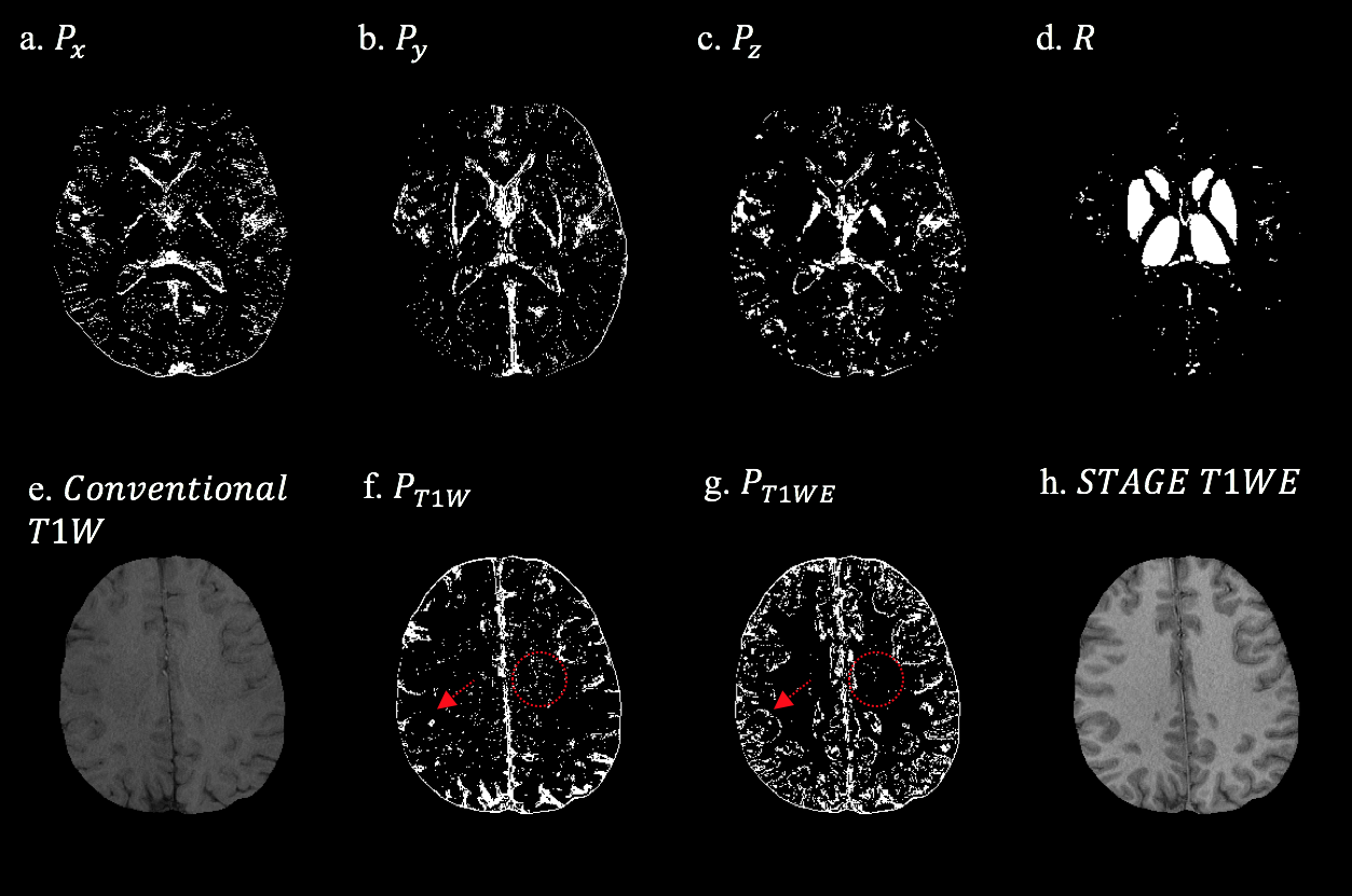
$$$W$$$ is proportional to the magnitude $$$\rho_m$$$. $$$R$$$ is zero in the high-susceptibility regions, vessels and basal ganglia, and one in other regions, to protect them from being over-smoothed. The basal ganglia structures are extracted from $$$\rho_m$$$, $$$\widehat{\chi}$$$(iSWIM), and T1WE data using an in-house developed atlas-based segmentation program. The vessels are extracted from $$$\widehat{\chi}$$$. $$$P$$$ is a binary edge mask derived from both $$$\widehat{\chi}$$$ and T1WE (Figure 1). Eq. 2 is solved using PCG. The stopping criteria is based on the standard deviation of the phase ($$$\sqrt{||\delta B_{(i)}-\delta B_{(i-1)}||_2^2/N}<\sigma_{\varphi}/\gamma B_0 TE$$$).

The proposed method was evaluated on both simulated⁽¹⁰⁾ and in vivo data from a 3T Siemens scanner including three double-echo scans (B₁:{ FA=6°, TR=25ms, TE_1=6.5ms, TE_2=17.5ms}, B₂:{ FA=24°, TR=25ms, TE_1=7.5ms, TE_2=18.5ms}, and B₃:{ FA=12°, TR=21ms, TE_1=2.5ms, TE_2=15ms}). The phase image was unwrapped using 3DSRNCP⁽¹¹⁾ and filtered using SHARP⁽¹²⁾. SCSWIM was compared to other methods such as TKD, iSWIM, and MEDI in terms of root mean squared error (RMSE) and structural similarity (SSIM) measures, using susceptibility model and COSMOS as the reference for the simulated and in vivo data. Susceptibilities of different basal ganglia structures and the internal cerebral vein (ICV) were measured.

Results

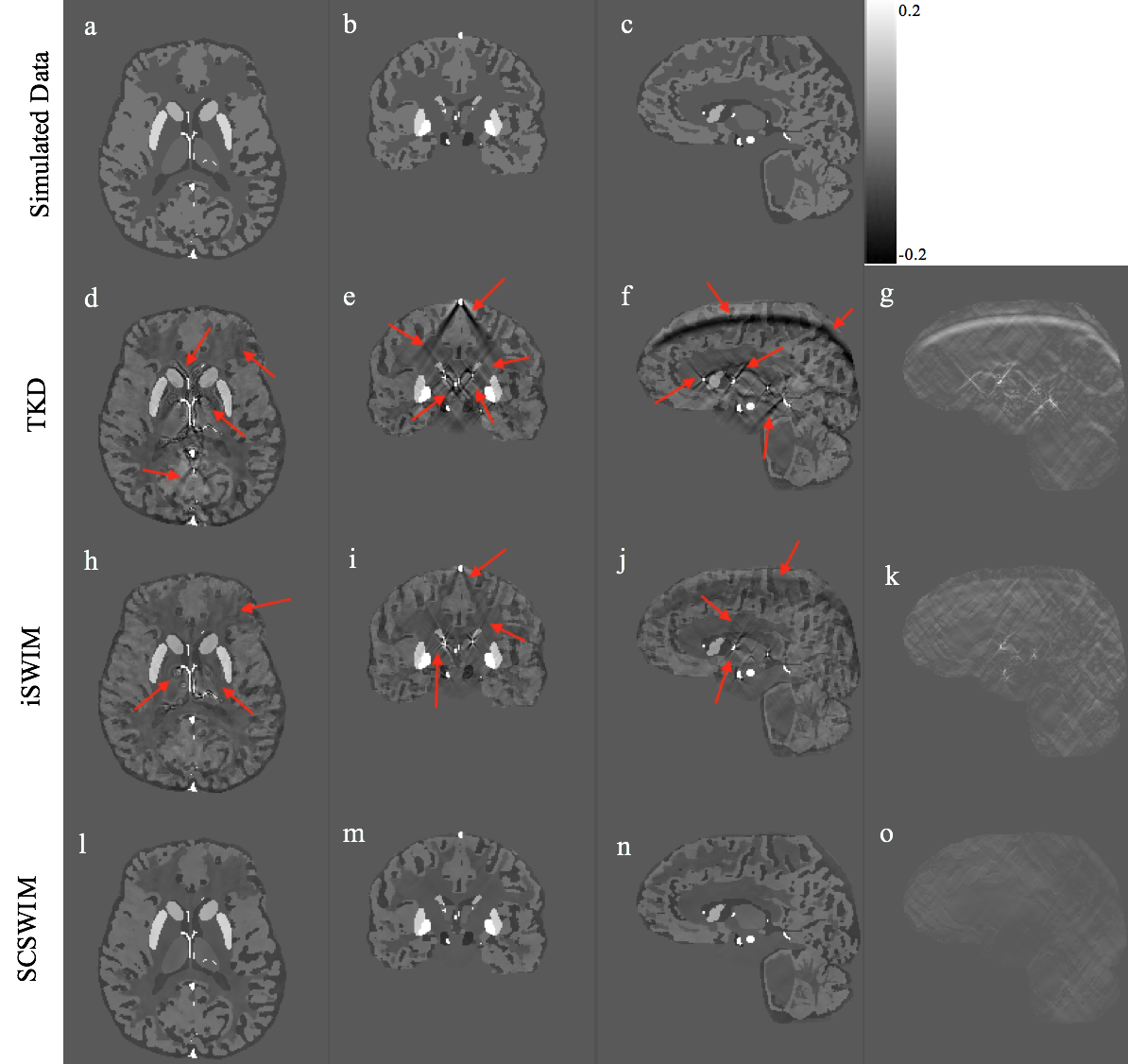
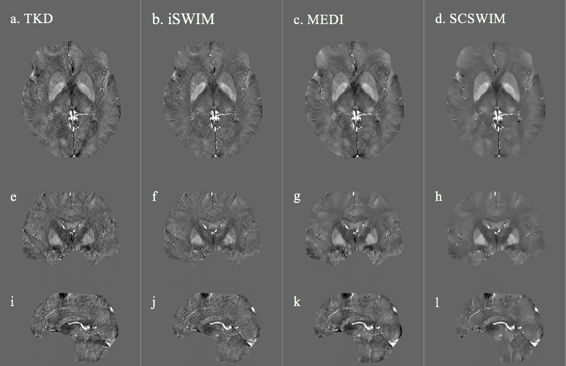
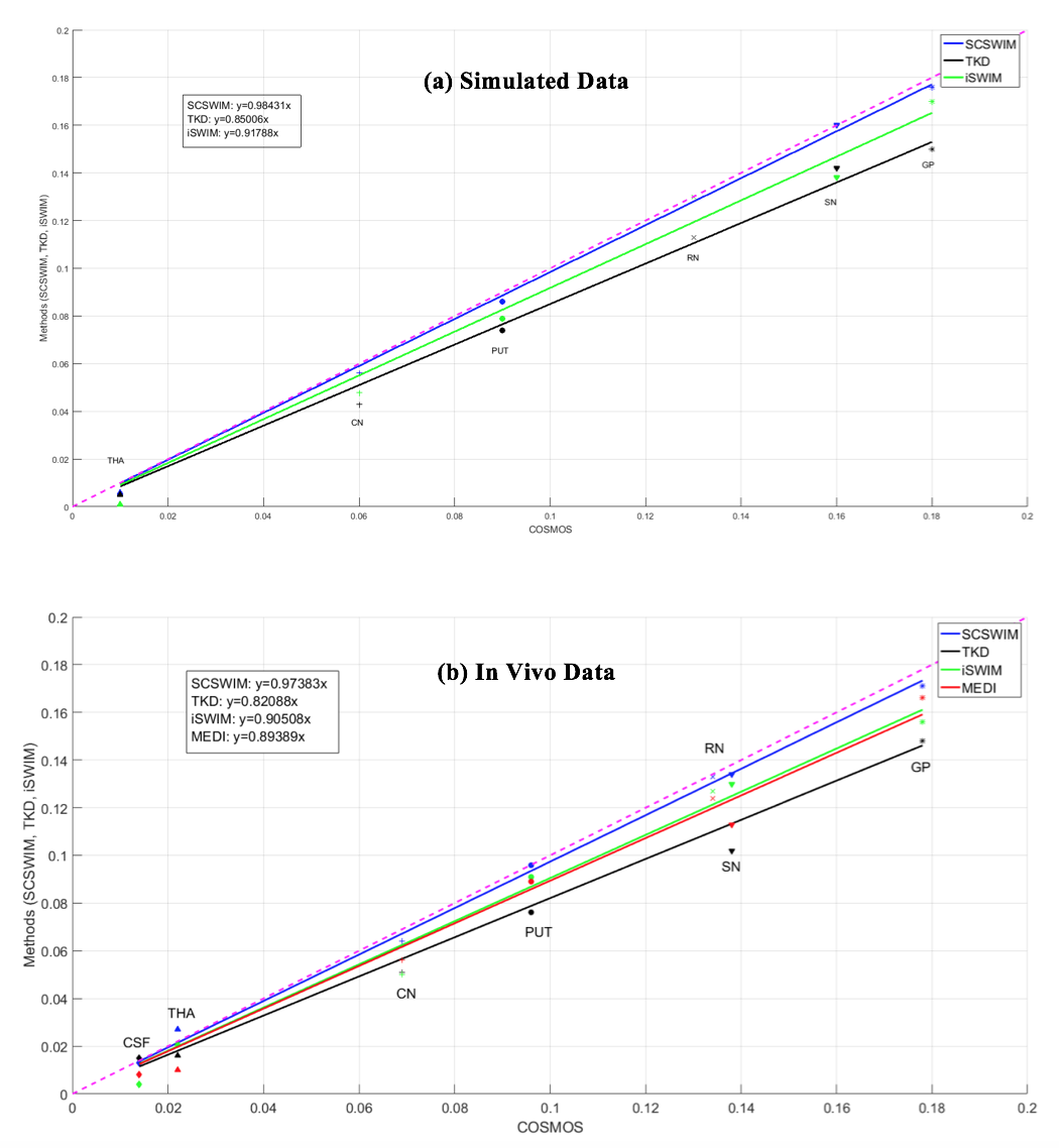
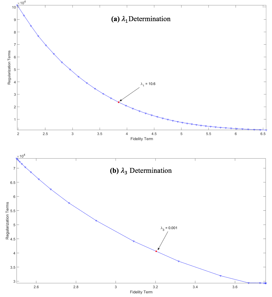
Simulations: Figure 1 shows the comparison between the constraints derived from regular T1 and STAGE T1WE in which STAGE provides more accurate and less noisy $$$P$$$ mask for WM/GM edges. Figure 2 shows the simulate model and reconstructed maps using different algorithms. The streaking artifacts (red arrows) were drastically reduced in SCSWIM. The measured RMSE and SSIM show that SCSWIM has the lowest error (0.005ppm) and the highest similarity to the model (97.85%) compared to other methods (TKD:0.014ppm,94.52% and iSWIM:0.011ppm,94.45%). The measured ICV susceptibilities in simulated data were: TKD:0.3384$$$\pm$$$0.075ppm, SCSWIM:0.442$$$\pm$$$0.002ppm and model: 0.45ppm. In vivo Data: Figure 3 shows that SCSWIM has less noise while the sharpness of the vessels and other structures are well-preserved. MEDI also provides a smooth reconstruction but some artifact has remained in regions close to veins. The measured ICV susceptibilities were: TKD:0.289$$$\pm$$$0.075ppm, MEDI:0.304$$$\pm$$$0.075ppm, SCSWIM:0.338$$$\pm$$$0.072ppm, and COSMOS:0.332$$$\pm$$$0.052ppm. Figure 4 shows that SCSWIM is highly correlated with COSMOS in basal ganglia. Figure 5 shows the effects of SCSWIM regularization parameters.

Discussion

The reconstructed image using SCSWIM has lower streaking artifacts and more accurate susceptibilities for basal ganglia and cerebral veins. This is mainly due to the utilization of the better contrast provided by the STAGE data. The current implementation of SCSWIM converges at the second iteration where the inner PCG loop can go up to 80 iterations. The reconstruction is significantly accelerated compared to the SFCR algorithm.

Conclusion

In this work, we have proposed a structurally constrained susceptibility reconstruction method which employs the unique contrast of STAGE imaging and segmented basal ganglia and vessels. SCSWIM leads to reduced streaking artifact, and better accuracy of the susceptibilities of both basal ganglia and veins compared to other methods.

Acknowledgements

No acknowledgement found.

References

1. Haacke EM, Liu S, Buch S, Zheng W, Wu D, Ye Y. Quantitative susceptibility mapping: current status and future directions. Magnetic Resonance Imaging. 2015; 33: p. 1–25.

2. Wharton S, Schafer A, Bowtell R. Susceptibility mapping in the human brain using threshold-based k-space division. Magnetic Resonance in Medicine. 2010; 63(5): p. 1292–304.

3. Tang J, Liu S, Neelavalli J, Cheng YC, Buch S, Haacke EM. Improving susceptibility mapping using a threshold- based k-space/image domain iterative reconstruction approach. Magn Reson Med. 2013; 69: p. 1396–407.

4. Liu J, Liu T, deRochefort L, Ledoux J, Khalidov I, Chen W, et al. Morphology enabled dipole inversion for quantitative susceptibility mapping using structural consistency between the magnitude image and the susceptibility mapping. NeuroImage. 2012; 59(3): p. 2560–2568.

5. Bao L, Li X, Cai C, Chen Z, van Zijl PCM. Quantitative susceptibility mapping using structural feature based collaborative reconstruction (SFCR) in the human brain. IEEE Transactions on Medical Imaging. 2016; 35(9): p. 2040–50.

6. Liu T, Spincemaille P, deRochefort L, Kressler B, Wang Y. Calculation of susceptibility through multiple orientation sampling (cosmos): a method for conditioning the inverse problem from measured magnetic field map to susceptibility source image in MRI. Magn Reson Med. 2009 Jan.; 61: p. 196–204.

7. Chen Y, Liu S, Wang Y, Kang Y, Haacke EM. Strategically acquired gradient echo (STAGE) imaging, part I: Creating enhanced T1 contrast and standardized susceptibility weighted imaging and quantitative susceptibility mapping. Magn Reson Imaging. 2018; 46: p. 130–139.

8. Wang Y, Chen Y, Wu D, Wang YWY, Sethi SK, Yang G, et al. Strategically acquired gradient echo (STAGE) imaging, part ii: Correcting for RF inhomogeneities in estimating T1 and proton density. Magn Reson Imaging. 2018; 46: p. 140–150.

9. Haacke EM, Reichenbach JR. Susceptibility Weighted Imaging in MRI: Basic Concepts and Clinical Applications: Wiley Blackwell; 2011.

10. Buch S, Liu S, Neelavalli J, Haacke EM. Simulated 3D brain model to study the phase behavior of brain structures. In Proceedings of the 20th Annual Meeting of ISMRM, (Melbourne, Australia); 2012. p. 2332.

11. Abdul-Rahman HS, Gdeisat MA, Burton DR, Lalor MJ, Lilley F, Moore CJ. Fast and robust three-dimensional best path phase unwrapping algorithm. Applied Optics. 2007; 46(26).

12. Schweser F, Deistung A, Lehr BW, Reichenbach JR. Quantitative imaging of intrinsic magnetic tissue properties using MRI signal phase: An approach to in vivo brain iron metabolism? NeuroImage. 2011; 54(4): p. 2789–807.

Figures

Figure 1. The first row shows the SCSWIM structural constraints for the in vivo data: (a-c) edge matrix, $$$P$$$, in three directions, and (d) structural matrix, $$$R$$$. The second row shows the advantage of extracting constraint from the STAGE vs conventional GRE: (g) conventional T1W, (h) STAGE T1WE, and the extracted edges (union of three directions) from (f) conventional T1W and (g) STAGE T1WE where (g) provides more information about the white and gray matter edges (red arrow) and it is less noisy (red circle) than (f). All figures except (e) and (h) are inverted for a better visualization.

Figure 2. This figure shows the axial, coronal and sagittal views of the susceptibility maps for the (a,b,c) ideal model, (d,e,f) TKD, (h,i,j) iSWIM and (l,m,n) SCSWIM. The streaking artifacts are shown in red arrows. Also, last column (g,k,o) shows the susceptibility error maps for different methods. The SCSWIM in the last row provides better reconstruction with less artifact and higher similarity to the ideal map in the first row.

Figure 3. Susceptibility maps from TKD, iSWIM, MEDI ($$$\lambda = 200$$$) and SCSWIM ($$$\lambda_1 = 10.6, \lambda_2 = \lambda_3 = 0.001$$$) methods are shown in the first, second, third and fourth columns, respectively. Three orthogonal views are shown in different rows. All of the images are displayed in the same windowing level.

Figure 4. These plots show the correlation of the susceptibilities of different basal ganglia structures in the reference image with the ones in the reconstructed images using different methods in the (a) simulated data and (b) in vivo data (TKD (black), iSWIM (green), MEDI (red) and SCSWIM (blue)). As it can be seen, SCSWIM is highly correlated with the reference image (model in the simulated data and COSMOS in the in vivo) in both plots.

Figure 5. SCSWIM parameter determination based on the fidelity $$$||W(\varphi/(\gamma B_0 TE)-F^{-1}DF\chi)||_2$$$ and regulations $$$||R\chi||_2+||PG\chi||_1$$$ terms. The optimal value are determined as $$$\lambda_1 = 10.6, \lambda_2 = \lambda_3 = 0.001$$$.

Proc. Intl. Soc. Mag. Reson. Med. 27 (2019)

4928