4926
QSM Inversion Through Parcellated Deep Neural Networks1Joint Department of Biomedical Engineering, Marquette University and Medical College of Wisconsin, Milwaukee, WI, United States, 2Department of Radiology, Medical College of Wisconsin, Milwaukee, WI, United States
Synopsis
Quantitative Susceptibility Mapping (QSM) can estimate tissue susceptibility distributions and reveal pathology in conditions such as Parkinson's disease and multiple sclerosis. QSM reconstruction is an ill-posed inverse problem due to a mathematical singularity of the requisite dipole convolution kernel. State-of-art QSM reconstruction methods either suffer from image artifacts or long computation times. To overcome the limitations of these existing methods, a deep-learning-based approach is proposed and demonstrated in this work. 200 QSM datasets were utilized to compare current QSM reconstruction methods (TKD, closed-form L2, and MEDI) with the proposed deep-learning approach using visual scoring assessment of streaking artifacts and image sharpness. These multi-reader study results showed that the deep learning solution can produce QSM images with improved scores in both streaking artifacts and image sharpness evaluation while providing an almost instantaneous inversion computation through neural network inferencing.
Purpose
Quantitative Susceptibility Mapping (QSM) can estimate tissue susceptibility distributions and reveal pathology such as Parkinson's disease and multiple sclerosis1. QSM reconstruction is an ill-posed inverse problem due to a mathematical singularity of the dipole kernel. State-of-art QSM reconstruction methods either suffer from image artifacts or long computation times, which limits QSM clinical translation efforts. To overcome these limitations of existing methods, a deep-learning-based approach is proposed.Methods
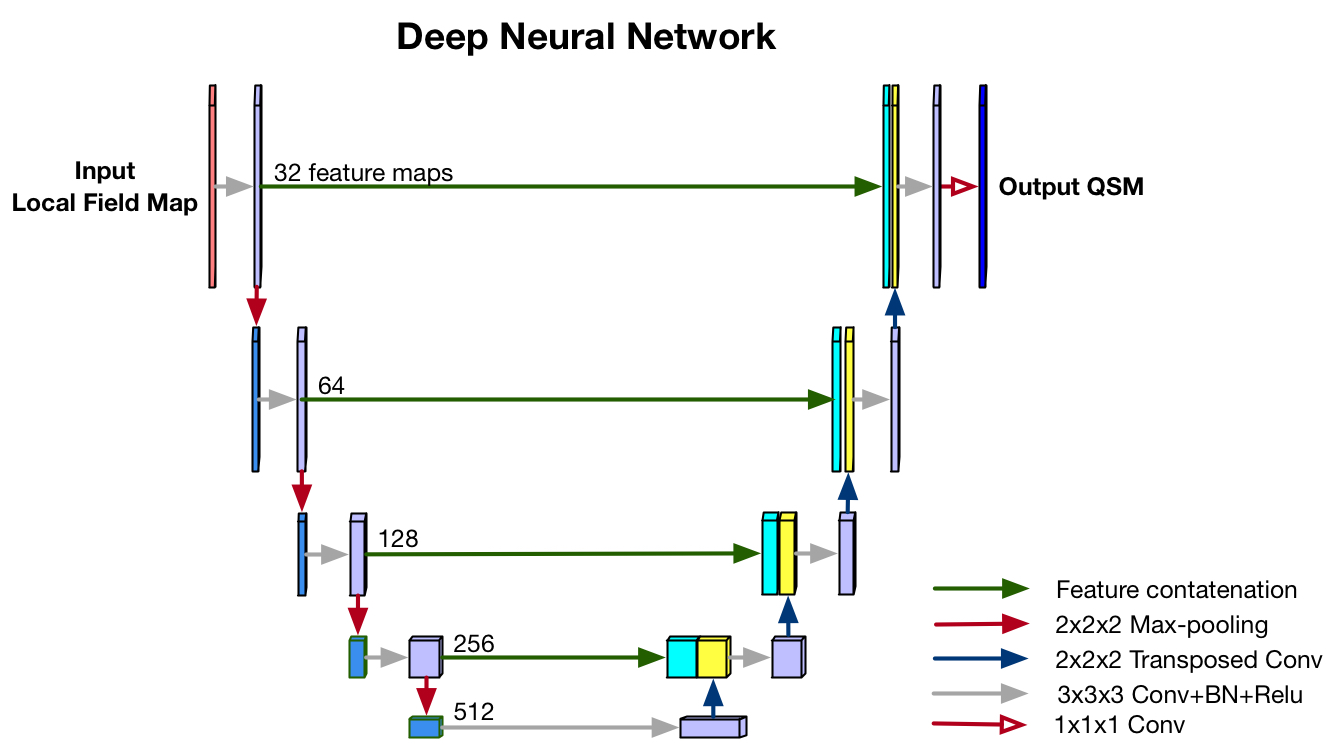
- Neural Network: A encoder-decoder neural network structure with skip connections was adopted, illustrated in Fig.1. The simulated susceptibility distributions were modeled to mimic the spatial frequency patterns of in-vivo brain susceptibility distributions. Spatial frequency power spectra were estimated using 50 QSM MEDI datasets. The simulated susceptibility maps were then generated using inverse Fourier transform of the square root of these cohort-averaged power spectral density estimates with element-wise random phase swaps. Forward field maps of the simulated susceptibility patches were used as the network input. The network was trained to independently invert 3D parcels of 192x192x64. In the prediction stage of the network, the whole tissue field volumes were segmented into 192x192x64 parcels with 32x32x32 overlap regions. After QSM inference using the trained network, the parcels were combined to form a composite image. To avoid edge artifacts in the combined QSM maps, 8x8x8 voxel boundaries were discarded before parcel combination. Linear regression utilizing the overlapping regions between blocks was used to adjust the relative scaling and bias between neighboring parcels. Final QSM maps were then computed via k-space substitution. A hard threshold of 0.2 was utilized to define the region of k-space where the forward field maps of the composite QSM estimation was substituted into the k-space of input field maps. This approach is denoted as ASPEN, standing for Approximated Susceptibility through Parcellated Encoder-decoder Networks.
- Datasets: 200 QSM datasets were acquired on high-school students with sports-related concussion and healthy controls at a 3T MRI scanner using commercially available SWI protocol with data acquisition parameters: in-plane data matrix = 320x256, FOV = 24 cm, voxel size = 0.5x0.5x2.0 mm3, TEs = [10.4, 17.4, 24.4, 31.4] ms, TR = 58.6 ms, autocalibrated parallel imaging factors = 3x1, acquisition time = 3.5 min. Complex multi-echo images were reconstructed from raw k-space data. The brain masks were obtained using the SPM tool. After background field removal using LBV method2, susceptibility inversion was performed using TKD3, closed-L24, MEDI5 and ASPEN. QSM toolbox6,7 was used to calculate TKD, closed-L2 and MEDI results.
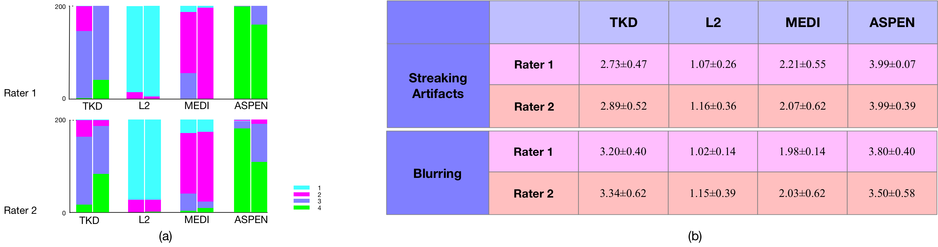
- Evaluation: Two raters were trained to perform ranking of each technique of the level of streaking artifacts and sharpness for 200 QSM datasets. The computed QSM maps were randomly displayed for each dataset. For streaking artifacts evaluation, four QSM maps were ranked from one to four, with four being the best appearing map. For sharpness, the maps were also ranked from one to four, with four being the sharpest map.
Results and Discussion
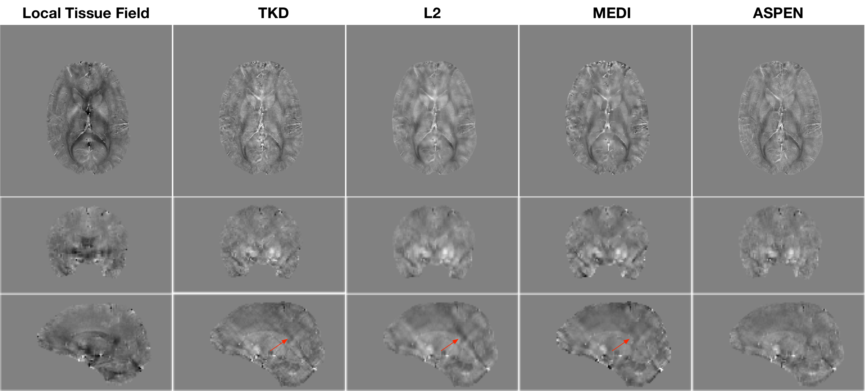
Fig.2 shows the QSM images of the four techniques in axial, coronal and sagittal views. Compared with TKD, L2 and MEDI, the ASPEN results show substantially reduced streaking artifacts, and preserve fine microstructures.
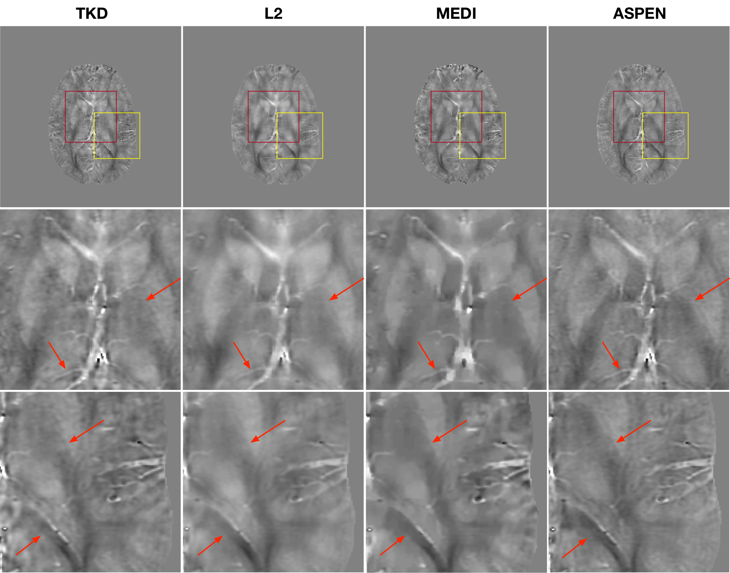
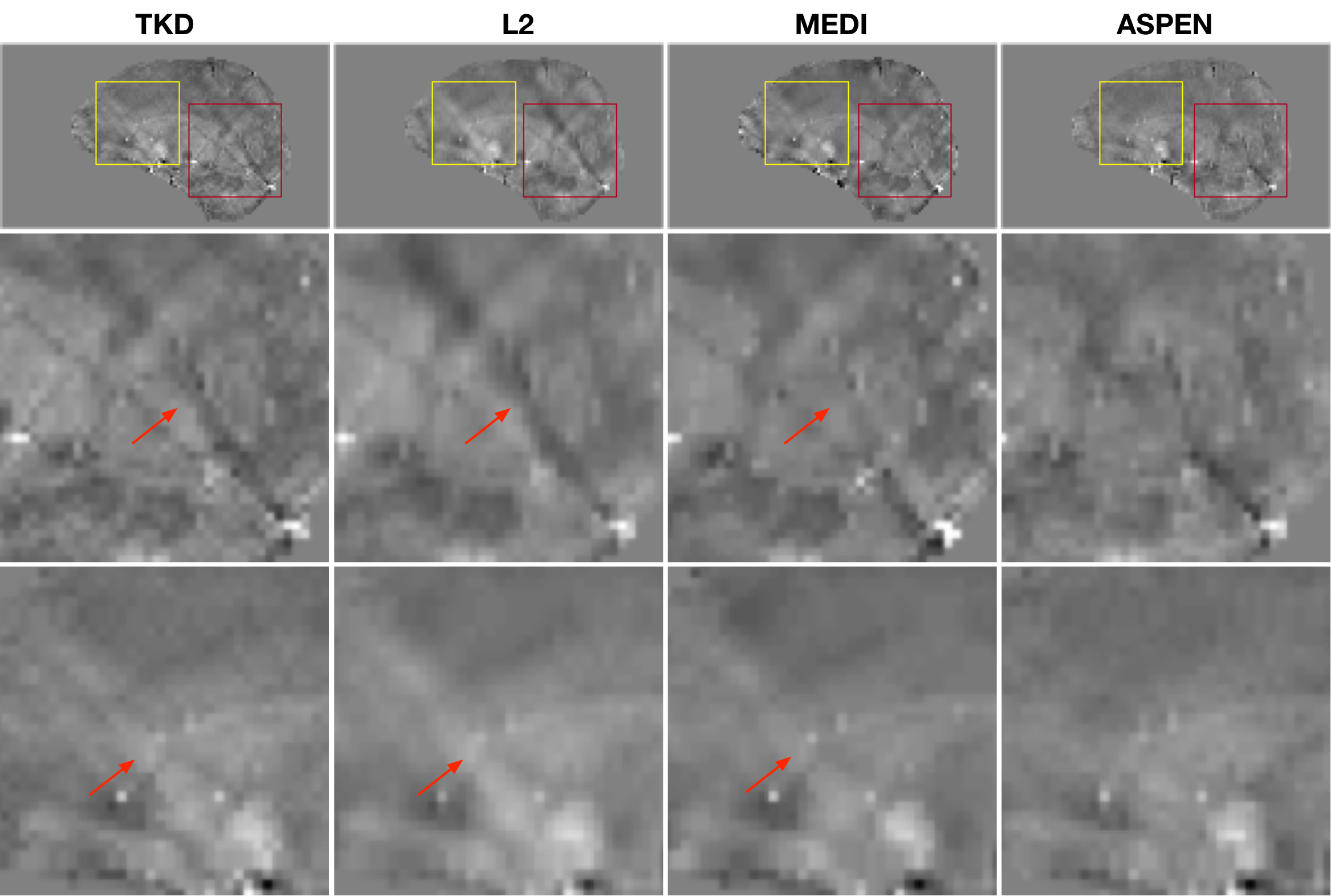
Fig.3 shows an axial view of the QSM maps, with the zoomed-in visualization clearly showing that the ASPEN map has the best sharpness. TKD shows compromised integrity at tissue boundaries. The closed-L2 and MEDI images have substantial image blurring due to their heavy use of spatial regularization to reduce streaking artifacts. In Fig.4, a sagittal view of QSM maps shows that ASPEN has minimal streaking artifacts, while other methods have clearly visible streaking artifacts.
Fig.5 shows the results of the multi-reader study. For streaking assessment, ASPEN achieved the highest score compared with other methods from two raters, indicating ASPEN can greatly suppress streaking artifacts. TKD received the second highest score in streaking artifacts assessment, followed by MEDI and closed-L2. For image sharpness assessment, ASPEN also achieved the highest score, TKD received the second highest score, followed by MEDI, closed-L2.
Conclusion
The proposed ASPEN approach requires no regularization or threshold parameter tuning and can infer susceptibility maps in near real-time on routine GPU hardware. The use of physics-based training for QSM neural networks opens a host of potential applications, whereby QSM can be tailored for specific applications and may allow improved utilization of QSM outside the brain.Acknowledgements
The authors would like to acknowledge Michael McCrea for sharing of concussion study QSM data.References
1. Wang Y, Liu T. Quantitative susceptibility mapping (QSM): decoding MRI data for a tissue magnetic biomarker. Magnetic resonance in medicine. 2015; 73 (1): 82-101.
2. Zhou D, Liu T, Spincemaille P, Wang Y. Background field removal by solving the Laplacian boundary value problem. NMR in Biomedicine. 2014; 27 (3): 312-319.
3. Wharton S, Schäfer A, Bowtell R. Susceptibility mapping in the human brain using threshold-based k-space division. Magnetic resonance in medicine. 2010; 63 (5): 1292-1304.
4. Bilgic B, Chatnuntawech I, Fan AP, et al. Fast image reconstruction with L2‐regularization. Journal of Magnetic Resonance Imaging. 2014; 40 (1): 181-191.
5. Liu J, Liu T, de Rochefort L, Ledoux J, et al. Morphology enabled dipole inversion for quantitative susceptibility mapping using structural consistency between the magnitude image and the susceptibility map. Neuroimage. 2012; 59(3): 2560-2568.
6. QSM Toolbox. http://pre.weill.cornell.edu/mri/pages/qsm.html.
7. Closed-form l2-Regularized QSM code. https://www.martinos.org/~berkin/software.html.
Figures