4907
Estimation of microstructural properties of white matter from multiple orientation GRE signal simulations of realistic models1Donders institute, Radboud university, Nijmegen, Netherlands
Synopsis
This study presents the creation of 2D white matter models, based on real histologically derived axon shapes, with
Introduction
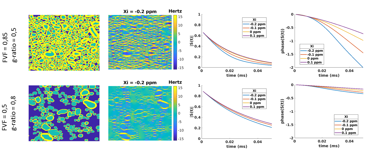
The gradient echo (GRE) MRI signal evolution is affected both in the magnitude and phase depending on the magnetic susceptibility of its various compartments with respect to the main static field B0. These effects have been successfully simulated with the hollow cylinder model [1]. However, recent work using realistic models of white matter has shown that this simple representation is not accurate enough to simulate the complex GRE signal [2]. In this study, we extend that work and present methods to: (i) generate models of white matter microstructure with different fiber volume fraction (FVF) and g-ratio based on real axon shapes; (ii) use these models to simulate GRE signal; (iii) train a deep learning network and demonstrate its ability to recover relevant microstructure specific parameters.Methods
Results
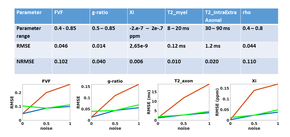
The network has demonstrated its ability to recover the parameters with a small error on the test dataset (see Fig 5), particularly when no noise was added neither during the training or on the evaluated signal. Even after adding 1% noise to the model, it was possible to successfully determine the susceptibility difference between myelin and the intra and extra axonal compartments as well as the g-ratio and the T2* of the free water compartment.Conclusion
Future work will evaluate if these realistic 2D models are a good representation of 3D model where fiber dispersion has to be accounted for. We have shown that some microstructural properties are recoverable using multiple orientation GRE data combined with prior axonal orientation knowledge. Future work will be devoted to the optimization of the sample rotations needed to ensure that the dictionary is better able to differentiate parameters. New parameter spaces will be searched to ensure that FVF and myelin water density, that are currently highly correlated, can be better teased apart. This approaches and deep learning decoding will then be applied to ex-vivo multi-echo data where that rotational freedom exists.Acknowledgements
This work is part of the research programme with project number FOM-N-31/16PR1056/RadboudUniversity, which is financed by the Netherlands Organisation for Scientific Research (NWO).References
[1] Wharton, Samuel, and Richard Bowtell. "Gradient echo based fiber orientation mapping using R2* and frequency difference measurements." Neuroimage 83 (2013): 1011-1023.
[2] Xu, Tianyou, et al. "The effect of realistic geometries on the susceptibility‐weighted MR signal in white matter." Magnetic resonance in medicine 79.1 (2018): 489-500.
[3] Cohen-Adad, et al. (2018, October 16). White Matter Microscopy Database. https://doi.org/10.17605/OSF.IO/YP4QG
[4] Zaimi, Aldo, et al. "AxonSeg: open source software for axon and myelin segmentation and morphometric analysis." Frontiers in neuroinformatics 10 (2016): 37.
[5] Mingasson, Tom, et al. "AxonPacking: an open-source software to simulate arrangements of axons in white matter." Frontiers in neuroinformatics 11 (2017): 5.
[6] Pajevic, Sinisa, and Peter J. Basser. "An optimum principle predicts the distribution of axon diameters in normal white matter." PLoS One 8.1 (2013): e54095.
[7] Liu, Chunlei. "Susceptibility tensor imaging." Magnetic Resonance in Medicine: An Official Journal of the International Society for Magnetic Resonance in Medicine 63.6 (2010): 1471-1477.
[8] Wharton, Samuel, and Richard Bowtell. "Fiber orientation-dependent white matter contrast in gradient echo MRI." Proceedings of the National Academy of Sciences (2012): 201211075.
[9] Chollet, François, et al. “Keras”, https://keras.io/
Figures
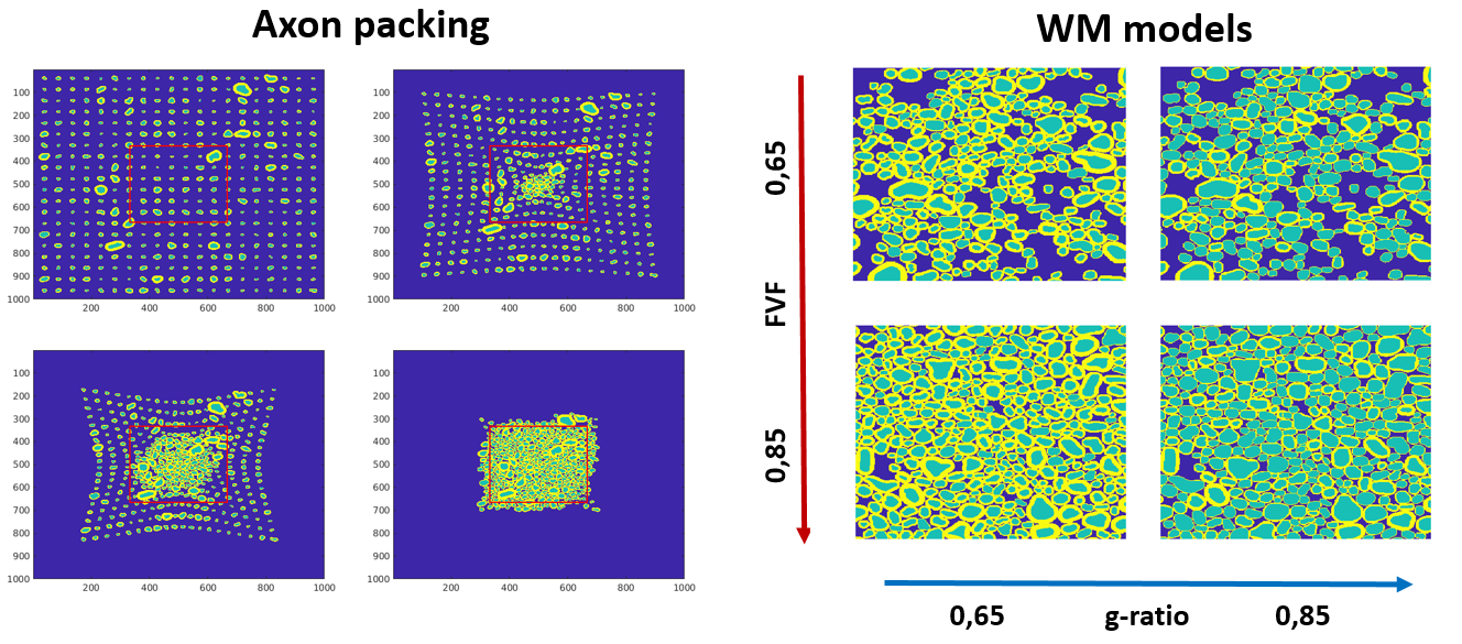
Fig 1. Left: Axon packing illustration. 400 axons randomly picked are regularly placed on a 1000x1000 grid, the extra-axonal space is represented in blue and the green axons are surrounded by their yellow myelin sheaths. The axons are attracted to the center of the image and repulse each other to avoid overlap. The packing process occurs to achieve a high FVF value (0,85).
Right: WM Models. Axons are randomly removed from the packed area to reach an expected FVF. Then, keeping the same myelinated axon shapes,the mean g-ratio is modified by dilatation/erosion of the myelin to obtain a model with expected FVF and g-ratio
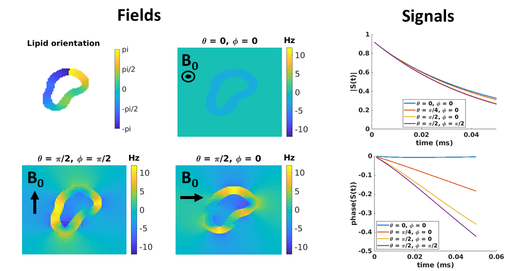
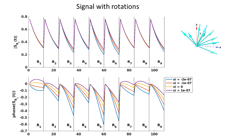
Fig 2. Left panel: Top left figure represent myelin phospholipid orientation of one axon. The 3 other images represent the simulated field with various B0 orientation (polar angle θ and the azimuthal angle Ф) and fixed susceptibility values (Xi = - 0,1 ppm, Xa = -0,1 ppm).
Right panel: Corresponding magnitude and phase of the signal with different θ and Ф values. As expected, there is an important signal variation as a function of θ, while the Ф has a smaller but non-negligible effect. This observation leads us to take the entire orientation of the B0 magnetic field (θ and Ф) into our model.