Synopsis

Quantitative mapping of myelin water fractions (MWF) can substantially improve our understanding of the progression of several demyelination white matter diseases such as multiple sclerosis. While MWF can be determined from both T2-weighted and T2*-weighted imaging data, it is much faster to collect T2*-weighted imaging data. However, estimation of MWF from T2*-weighted imaging data using a multi-exponential component model is an ill-conditioned problem whose solutions are often very sensitive to noise and modeling errors. In this work, we address this problem using a new model-based method. This method is characterized by: a) absorbing the spectral priors using the Bayesian-based statistical framework, and b) absorbing the spatial priors using a reproducing kernel based model. Both simulation and experimental results show the proposed method significantly outperforms the conventional parameter estimation methods currently used for MWF estimation.

Introduction

Method

A common model used for MWF estimation decomposes the T2*-weighted imaging data into three exponential components^3-5:

$$\hspace{18em}\rho(\boldsymbol{x}_p,t)=\sum_{l=1}^3A_{\ell}(\boldsymbol{x}_p)e^{-t/T_{2,\ell}^{*}(\boldsymbol{x}_p)}e^{i2{\pi}f_{\ell}(\boldsymbol{x}_p)t},\hspace{18em}\quad\quad(1)$$

which correspond to the water within the myelin sheath, myelinated axons and all others tissues. $$$A_{\ell}(\boldsymbol{x}_p)$$$, $$$T_{2,\ell}^{*}(\boldsymbol{x}_p)$$$ and $$$f_{\ell}(\boldsymbol{x}_p)$$$ denote the amplitude (related to concentration), $$$T_2^*$$$ relaxation time constant and frequency shift of each component at location $$$\boldsymbol{x}_p$$$ ($$$p=1,2,...,P$$$). Accurate signal decomposition based on Eq. (1) is challenging due to ill-conditonedness. Here, we address this issue by incorporating both spectral and spatial prior information.

Incorporation of spectral priors

Spectral priors are incorporated using the Bayesian-based statistical framework. More specifically, we estimate the nonlinear spectral parameters (i.e., $$$\{T_{2,\ell}^{*}\}$$$ and $$$\{f_{\ell}\}$$$) in two steps.

Firstly, we obtain the initial estimates of $$$\{T_{2,\ell}^{*}\}$$$ and $$$\{f_{\ell}\}$$$ using the conventional parameter estimation methods (we denote the solution as $$$\{\bar{T}_{2,\ell}^{*}\}$$$ and $$$\{\bar{f}_{\ell}\}$$$ ) and then approximate their empirical distributions using a Gaussian model:

$$\text{Prob}(T_{2,\ell}^*){\approx}\mathcal{N}(\mu_{T_{2,\ell}^{*}},\sigma_{T_{2,\ell}^{*}}^{2})\quad\text{and}\quad\text{Prob}(f_{\ell}){\approx}\mathcal{N}(\mu_{f_{\ell}},\sigma_{f_{\ell}}^{2}).$$

Secondly, we re-estimate the nonlinear parameters, incorporating the empirical prior distributions $$$\text{Prob}(T_{2,\ell}^*)$$$ and $$$\text{Prob}(f_{\ell})$$$ via the Bayesian-based statistical framework:

$$\tilde{T}_{2,\ell}^{*}=\arg\min_{T_{2,\ell}^*}\sum_{p=1}^{P}||\bar{T}_{2,\ell}^*(\boldsymbol{x}_p)-T_{2,\ell}^*(\boldsymbol{x}_p)||_2^2+\lambda_{T_{2,\ell}^*}||T_{2,\ell}^*(x_p)-\mu_{T_{2,\ell}^*}||_2^2$$

$$\tilde{f}_{\ell}=\arg\min_{f_{\ell}}\sum_{p=1}^{P}||\bar{f}_{\ell}(\boldsymbol{x}_p)-f_{\ell}(\boldsymbol{x}_p)||_2^2+\lambda_{f_{\ell}}\sum_{p=1}^P||f_{\ell}(x_p)-\mu_{f_{\ell}}||_2^2.$$

Incorporation of spatial priors

Once the nonlinear parameters have been determined, we estimate the linear coefficients $$$\{A_{\ell}(\boldsymbol{x}_p)\}$$$ for all the voxels jointly, incorporating spatial priors. To this end, we use a kernel-based model to represent $$$A_{\ell}(\boldsymbol{x}_p)$$$, leveraging our previous work in this area⁶. More specifically, we assume $$$A_{\ell}(\boldsymbol{x}_p)$$$ can be viewed as a nonlinear function of a set of low-dimensional features $$$\boldsymbol{z}_p{\in}{\mathbb{R}^n}$$$ derived from prior images (e.g., T1W images). While such a nonlinear function is often highly complex in practice, we can linearize it in a high-dimensional transformed space using the “kernel trick” in machine learning:

$$\hspace{22.3em}A_{\ell}(\boldsymbol{x}_p)=\sum_{q=1}^P\alpha_{\ell,q}k(\boldsymbol{z}_q,\boldsymbol{z}_p),\hspace{22.3em}\quad(2)$$

where $$$k(\cdot,\cdot)$$$ is some kernel function. Substituting Eq. (2) into Eq. (1) leads to the kernel-based representation for the T2*-weighted imaging data:

$$\hspace{16.5em}\rho(\boldsymbol{x}_p,t)=\sum_{\ell=1}^3\left\{\sum_{q=1}^P\alpha_{\ell,q}k(\boldsymbol{z}_q,\boldsymbol{z}_p)\right\}e^{-t/T_{2,\ell}^{*}(\boldsymbol{x}_p)}e^{i2{\pi}f_{\ell}(\boldsymbol{x}_p)t}.\hspace{16.5em}\quad(3)$$

To determine the $$$\{\alpha_{\ell,q}\}$$$ in Eq. (3), we choose the radial Gaussian kernel function and fit the kernel-based model to the measurements by solving a linear least-squares optimization problem that takes into account all the voxels jointly. Once the $$$\{\alpha_{\ell,q}\}$$$ have been estimated, we can reconstruct $$$A_{\ell}(\boldsymbol{x}_p)$$$ based on Eq. (2), which will yield the desired MWF maps^3-5.

Results

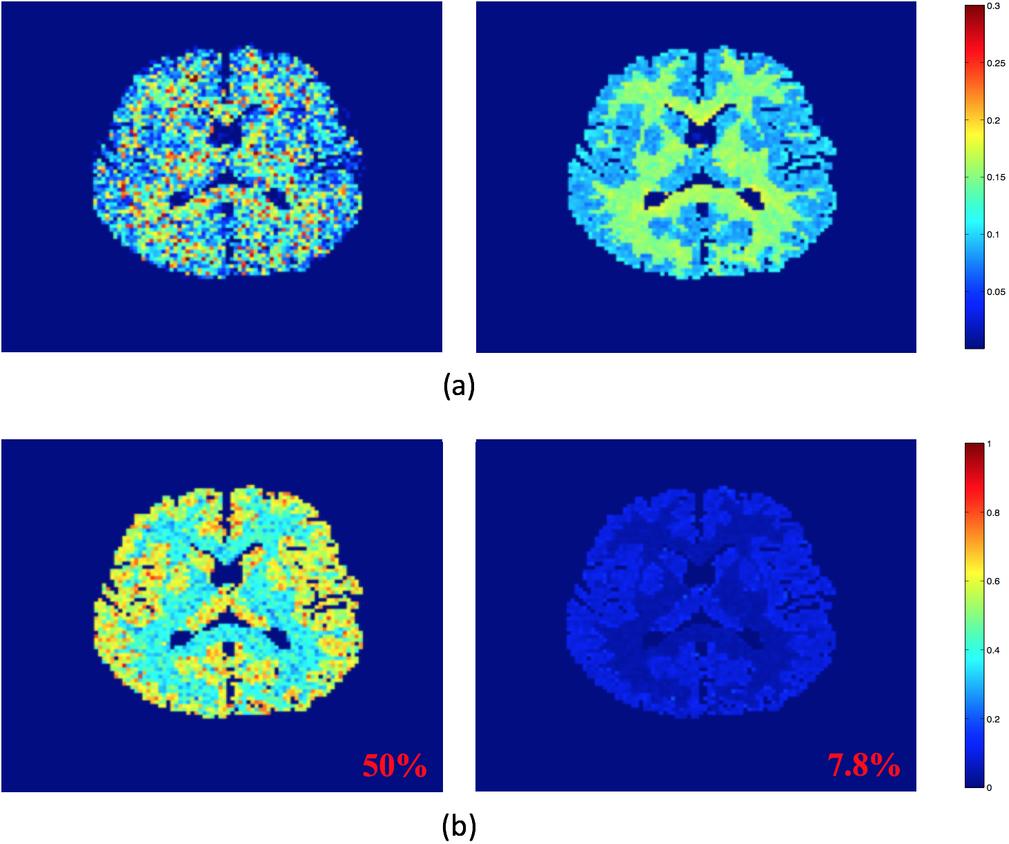
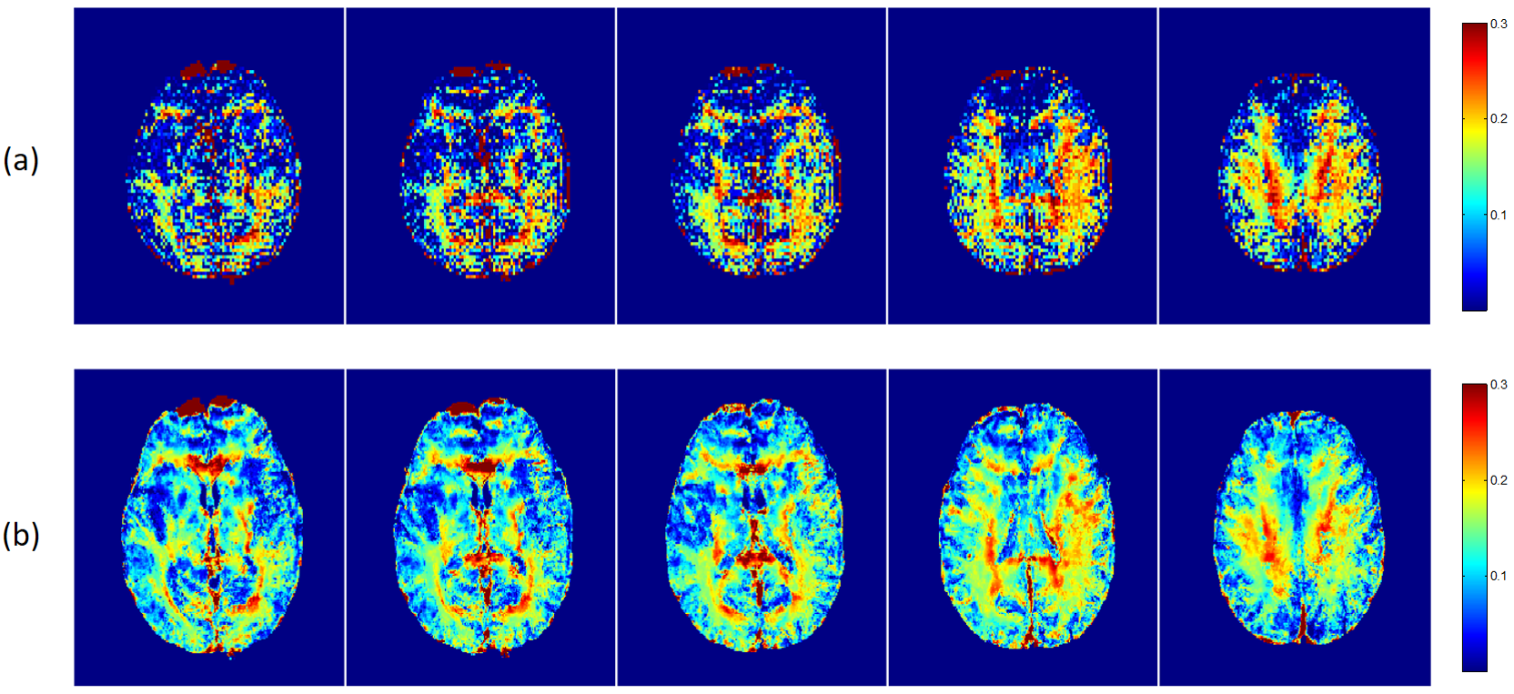
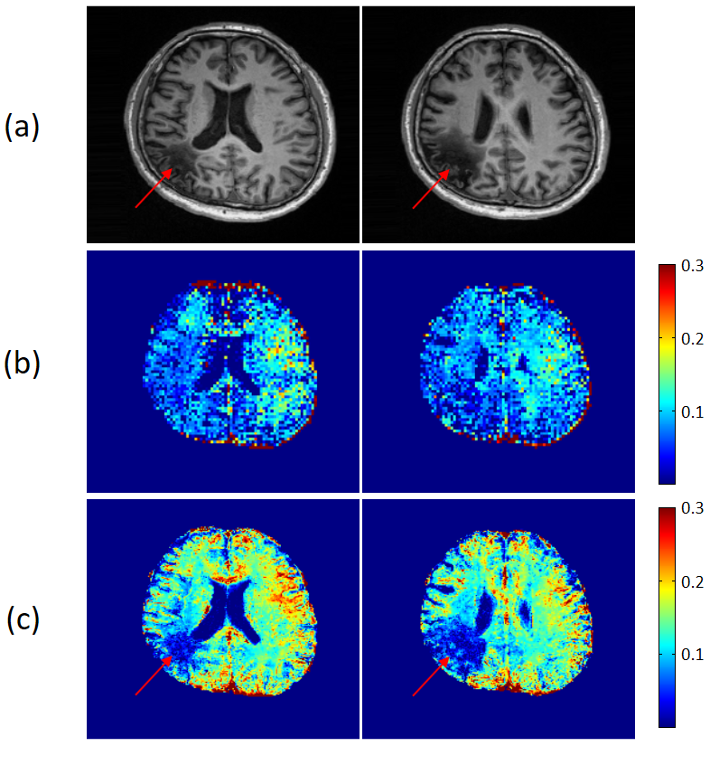
The performance of the proposed method has been evaluated using both simulated and experimental data. In our Monte-Carlo simulation study, the simulated data were generated based on Eq. (1) using published literature values³ for the spectral parameters and in vivo levels of additive Gaussian white noise. Figure 1 shows the estimation standard deviation from the Monte-Carlo study and the MWF maps estimated from one of the 40 realizations. As can be seen, the MWF estimates obtained using the proposed method show significantly reduced errors and estimation variances. In our experimental study, in vivo data were collected on a 3T scanner using a multi-gradient-echo sequence. Two sets of representative results are shown in Fig. 2 and 3, one from a healthy subject (Fig. 2) and the other from a patient with a chronic stroke (Fig. 3). As can be seen, the MWF maps produced by the proposed method show significantly reduced artifacts and estimation variations over those obtained using the conventional scheme, which is consistent with those from our simulation study.

Conclusions

Acknowledgements

References

[1] MacKay AL, Laule C. Magnetic resonance of myelin water: an in vivo marker for myelin. Neural Plast. 2016;2(1): 71-91.

[2] Alonso‐Ortiz E, Levesque IR, Pike GB. MRI‐based myelin water imaging: A technical review. Magn Reson Med. 2015;73(1): 70-81.

[3] Du YP, Chu R, Hwang D, et al. Fast multislice mapping of the myelin water fraction using multicompartment analysis of T2* decay at 3T: A preliminary postmortem study. Magn Reson Med. 2007;58(5):865-870.

[4] Hwang D, Kim DH, Du YP. In vivo multi-slice mapping of myelin water content using T2* decay. NeuroImage. 2010;52(1):198-204.

[5] Nam Y, Lee J, Hwang D, et al. Improved estimation of myelin water fraction using complex model fitting. NeuroImage. 2015;116:214-221.

[6] Li Y, Liang ZP. Constrained image reconstruction using a kernel+sparse model. Proc Intl Soc Magn Reson Med. 2018;p. 657.