4899
Feasibility study on artificial neural network based myelin water fraction mapping1Department of Electrical and Electronic Engineering, Yonsei University, Seoul, Korea, Republic of, 2Seoul St.Mary's Hospital, The Catholic University of korea, Seoul, Korea, Republic of, 3Department of Radiology and Research Institure of Radiological Science, Severance Hospital, Yonsei University College of Medicine, Seoul, Korea, Republic of, 4Department of Radiology, Inje University College of Medicine, Haeundae Paik Hospital, Busan, Korea, Republic of
Synopsis
We developed an artificial neural network (ANN) using magnitude 3-pool signal model based training sets. Simulations were performed for evaluation with various SNR and
Introduction
Previous studies demonstrated Myelin Water Fraction (MWF) mapping using multi pool fitting on multi-echo Gradient echo (mGRE) acquisitions1,2. Due to the many parameters required for fitting, these methods required long processing time and were vulnerable to noise and deviations from the model. Here, we applied artificial neural network (ANN) which has been demonstrated to supplement these shortcomings3.Method
1. Dataset
[Numerical Dataset]
Training dataset: 100,000 mGRE data were generated for the train-set using the parameters in $$ S_1(TE) = A_{my}*e^{-(1/T_{2,my}^{*})TE}+A_{ax}*e^{-(1/T_{2,ax}^{*})TE}+A_{ex}*e^{-(1/T_{2,ex}^{*})TE} ]$$ Specifically, the simulated signal was composed of three pool exponential signal with echo spacing of 1ms. Amy, Aax, Aex denote the amplitudes of myelin water, intracellular water, and extracellular water pools. T2*,my, T2*,ax, T2*,ex are the T2* values of corresponding pools.
Testing dataset: For evaluation, a numerically simulated dataset was generated with the specification of Fig. 2. (d),(e).
[In-vivo data]
We acquired mGRE images from 2 subjects for testing. Specifically, Subject 1 was a healthy volunteer and Subject 2 was a patient with genetically confirmed X-linked adrenoleukodystrophy (X-ALD) disease. The imaging parameters for mGRE images were: TR=60ms, TE1=1.6ms, ΔTE=1ms, field of view =256×256×100mm3, spatial resolution = 1.6×1.6×2.0mm3. or Subject 2, an additional ihMT (magnetization transfer) imaging protocol was acquired for this subject and quantitative ihMT(qihMT) was generated from ihMT data (marked as MT in Figure 5.(d) )
2. Network Design
The neural network for the training was composed of 5 layers as shown in Fig. 1.
3. Evaluations
Simulations were performed to compare the performance of the ANN regarding the two aspects with conventional 3-pool model fitting2,4. Also, visual comparison for in-vivo results was performed.
Robustness to noise: Performance was compared to various SNR levels (50, 150, 300) (Fig. 2. (d)).
Robustness to deviation from the model: Simulated data were compared assuming ΔB0 slice inhomogeneity as5 $$ S_2(TE)= S_1(TE)*sinc(\gamma G_z \frac{\triangle z}{2}TE)$$ Here, γ is the gyromagnetic ratio, GZ is the linear approximation of the field gradient in the slice-select direction, and ∆z is the slice thickness.
Ranges of the parameters for the simulation data are shown in Fig. 2. (e).
In-vivo application: The method was further applied voxel-wise for in-vivo images, which were not included in the training set. The processing time was measured. We used Intel Core I7-7500U CPU while the ANN model was processed by one GeForce GTX 1080 TI GPU with 11GB memory.
Results
Figure 3 shows the comparison results for various SNR levels (N=500) (a-c). Figure 3. (d) shows box-plot of the overall results. Using ANN shows decreased mean error compared to the fitting method (from 3.48 to 2.01) and decreased standard deviation (from 3.26 to 1.31). Figure 4 shows results for different levels of slice ΔB0 inhomogeneity (GZ). While fitting method shows apparent bias for increased GZ, the ANN method was relatively more stable. In-vivo data are shown in Fig. 5. Figure 5. (a) and (b) are images from the healthy volunteer and (c) and (d) from the patient. Particularly, the MT image shows decreased myelin in the genu region which is also visible in the ANN model. Processing time for the ANN took less than 0.5 seconds, while the fitting method took over 60 seconds.Conclusion and Discussion
ANN based MWF mapping showed reduced mean error and standard deviation compared to the fitting method and were more robust to different GZ, which may reflect the deviation from the model. In-vivo results of the ANN model also showed improved image quality, even though training was performed with simulation data only. Moreover, the ANN model is more time efficient than the fitting method, which may be beneficial for clinical application.
There are some limitations in our current study. The network seems to slightly overestimate MWF values within 10 to 20 and underestimate the values over 20. Similar behaviors were observed in 6 and might be due to the limitations of our model architecture. Moreover, in the current study, only simulation data was used for the training, which does not yet reflect situations in real in-vivo data such as susceptibility anisotropy, motion, and flow etc7. Thus adding in-vivo data for the training set may be beneficial.
Acknowledgements
This research was supported by Basic Science Research Program through the National Research Foundation of Korea(NRF) funded by the Ministry of Science, ICT and future Planning (NRF-2016R1A2B3016273)References
1. Du YP, Chu R, Hwang D, Brown MS, Kleinschmidt-DeMasters BK, Singel D, Simon JH. Fast multislice mapping of the myelin water fraction using multicompartment analysis of T2* decay at 3T: a preliminary postmortem study. Magn Reson Med 2007;58(5):865-870.
2. Hwang D, Kim D-H, Du YP. In vivo multi-slice mapping of myelin water content using T2* decay. Neuroimage 2010;52(1):198-204.
3. Golkov, V., et al., q-Space Deep Learning: Twelve-Fold Shorter and Model-Free Diffusion MRI Scans.IEEE Transactions on Medical Imaging, 2016. 35(5): p. 1344-1351.
4. Lee H, Nam Y, Kim D-H, Echo-Time Range Effects on Gradient Echo Based Myelin Water Fraction Mapping at 3T, Magn Reson Med 2018.
5. Alonso-Ortiz E, Levesque IR, Paquin R, Pike GB, Field inhomogeneity correction for gradient echo myelin water fraction imaging, Magn Reson Med 2017:78(1):49-57.
6. Ouri Cohen, Bo Zhu, Matthew S. Rosen, MR fingerprinting Deep RecOnstruction NEtwork (DRONE), Magn Reson Med 2018:80(3):885-894.
7. Lee H, Nam Y, Lee HJ, Hsu JJ, Henry RG, Kim DH, Improved three-dimensional multi-echo gradient echo based myelin water fraction mapping with phase related artifact correction, Neuroimage 2018:169:1-10.
Figures
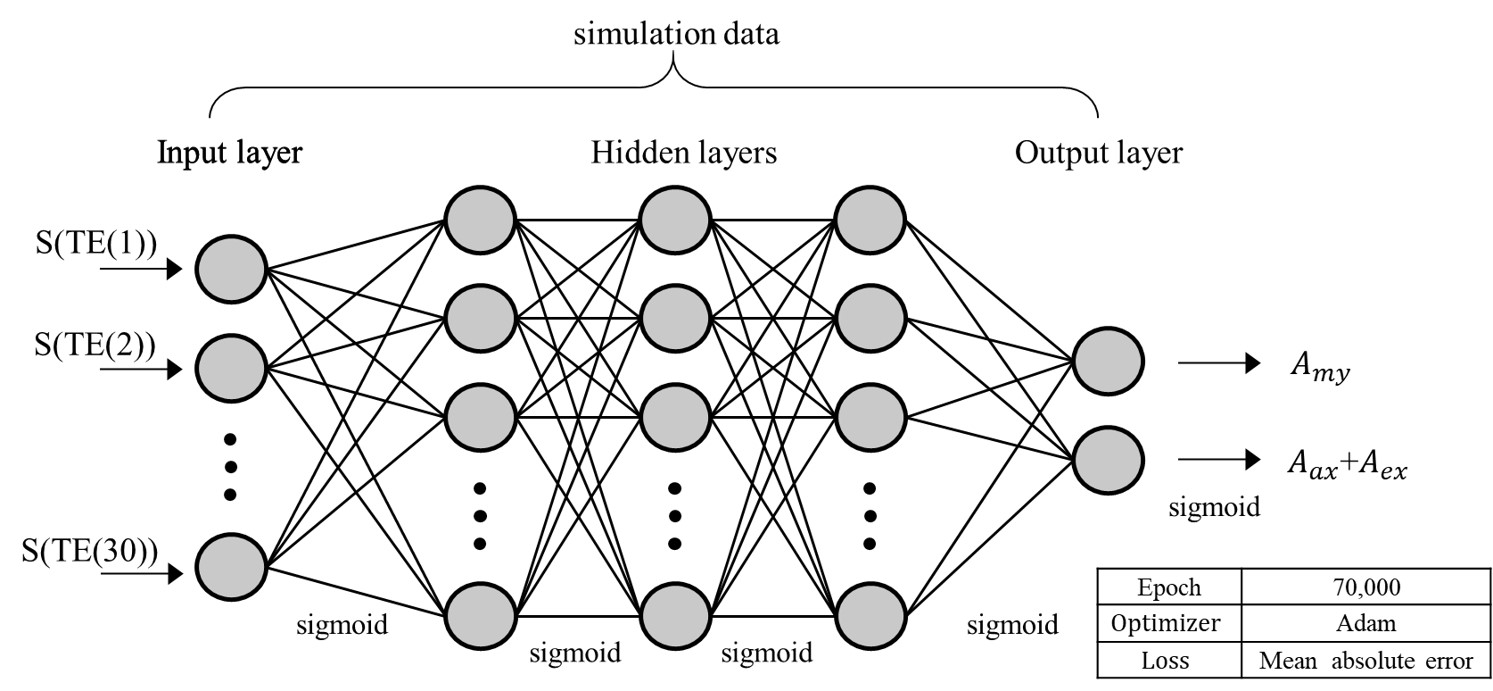
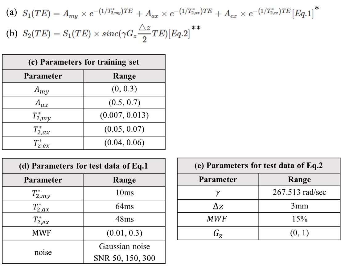
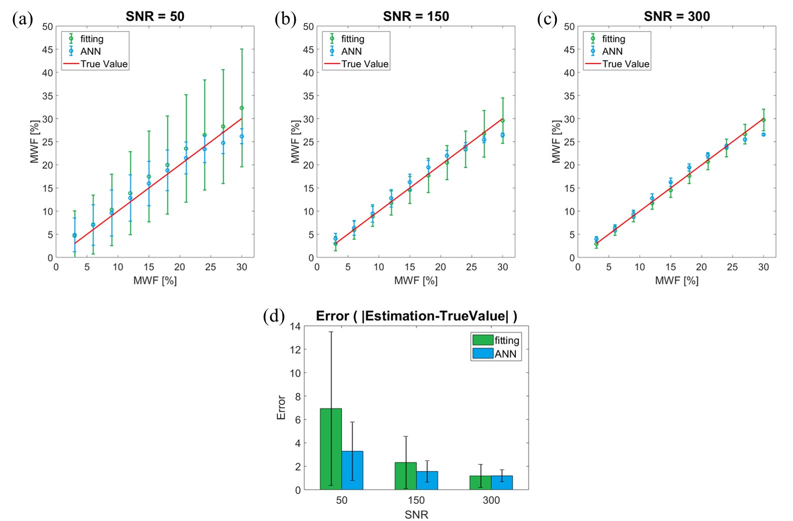
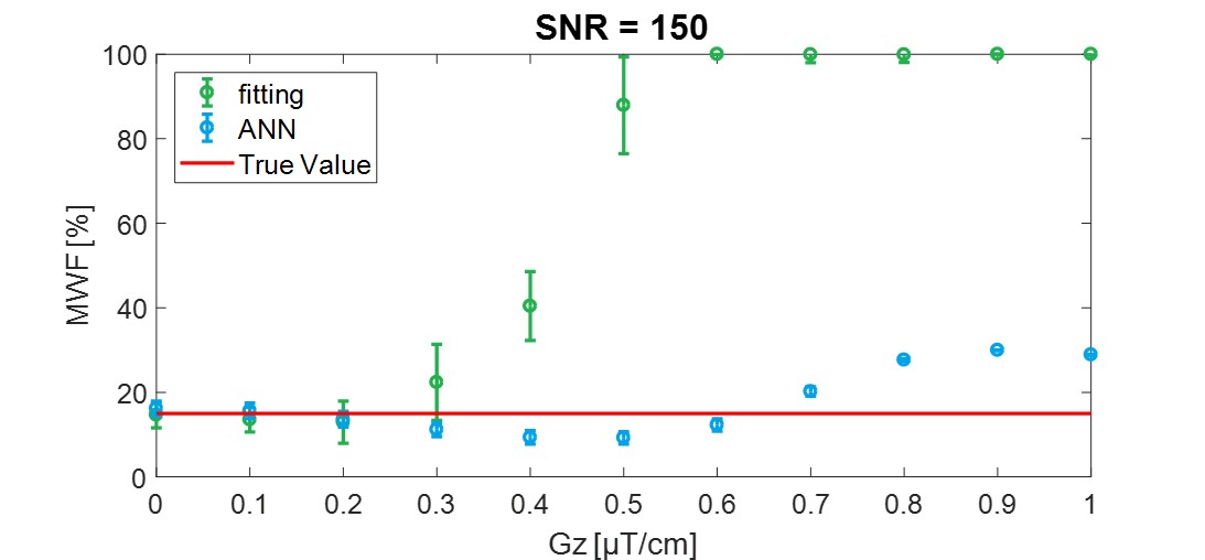
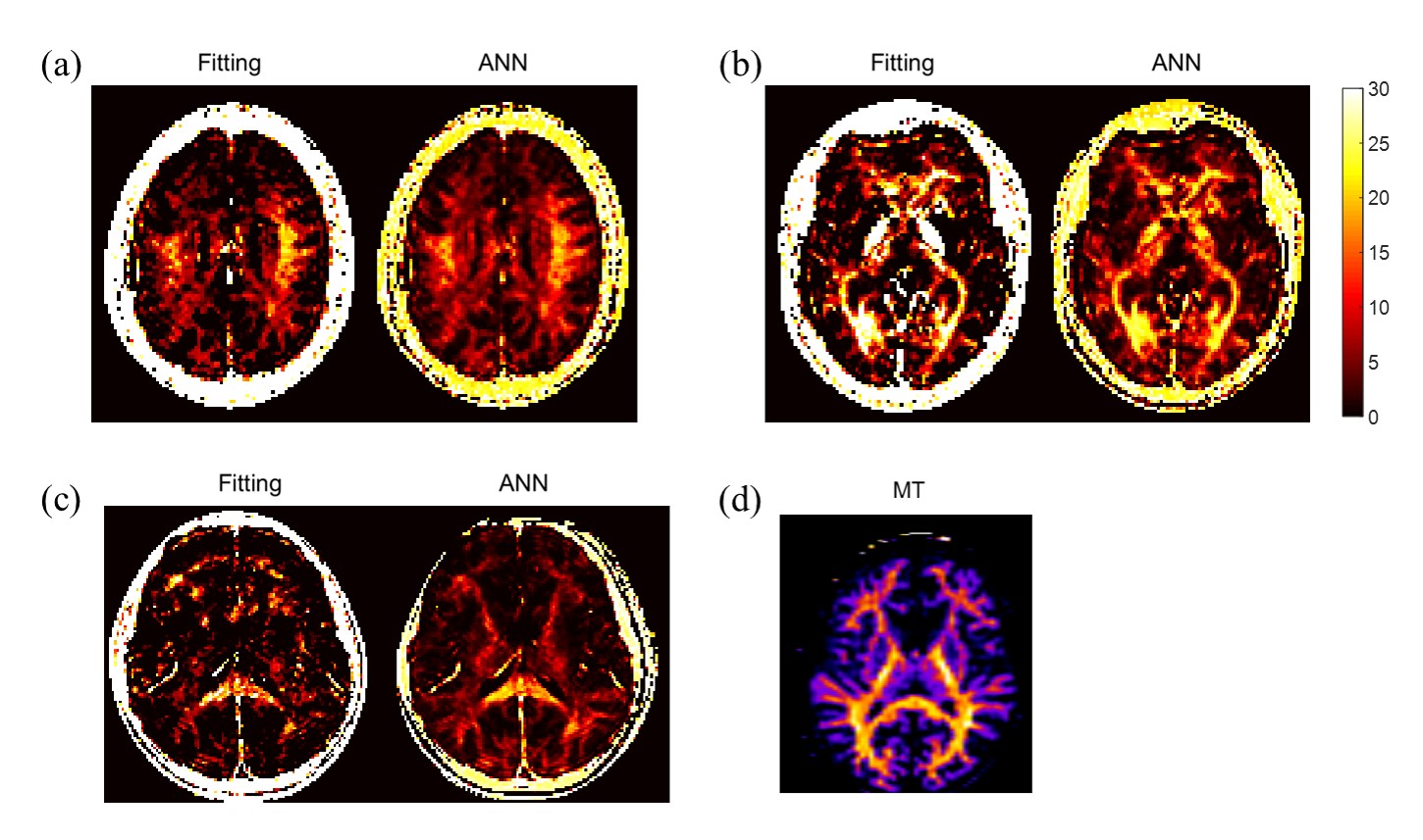
Figure 5. Resultant image of directly applying the trained model to in-vivo images. Resultant images from two methods (fitting and ANN) are shown. (a), (b) are images from the healthy volunteer (Subject 1). (c) is images of the patient (Subject 2). For Subject 2, an additional image from qihMT is shown (d).