4893
Tools for assessing and mitigating confounding effects in Machine-Learning based studies of MRI data1INFN, sez. Pisa, Pisa, Italy, 2Scuola Normale Superiore, Pisa, Italy, 3University of Pisa, Pisa, Italy
Synopsis
Using Machine Learning (ML) techniques on neuroanatomical data obtained with magnetic resonance imaging (MRI) is becoming increasingly popular in the study of Psychiatric Disorders (PD). However, this kind of analyses can be affected by overfitting and thus be sensitive to biases in the dataset, producing hardly reproducible results. It is therefore important to identify and correct possible bias sources in the sample. We present two tools aimed at addressing this matter: a methodology to assess the confounding power of a variable in a specific classification task, and a cost function to use during classifier training on highly biased data.
INTRODUCTION
In the latest MRI-based ML studies1, the awareness of potential sources of uncontrolled variation (especially those related to the MRI acquisition sites2) and of the difficulties in normalizing these data is growing. This motivates researchers to limit their analyses to a few sites and homogeneous groups of subjects, sacrificing sample size. However, it is not always clear which variables must be considered during dataset stratification to avoid confounding biases. Furthermore, even when all the confounding factors are known, it is difficult to isolate a group of subjects that are adequately homogeneous with respect to all of them. To tackle this problem, ML approaches have been proposed that aim at minimizing a saddle-shaped cost function during training3. This function represents the compromise between optimizing classification performances while avoiding to learn from bias-generated differences. However, when the value of a confounding variable and the class label are highly correlated within subjects, this tug of war risks hampering the classifier ability to actually learn anything. In this study we present a cost function that improves the probability of learning the correct classification pattern in unbalanced datasets overcoming these difficulties. Furthermore, a practical method for assessing the confounding effect of a variable is introduced.
CONFOUNDING POWER INDEX
To study the confounding power CPx of a categorical variable $$$X\in\{0,1\}$$$ we propose to measure the effect that a strong bias (related to X) in the dataset has in a two-group classification. To this purpose, a classifier must be trained on three different dataset configurations (see figure 1). From the relationship in the white box, an index to quantify the confounding power can be derived as:
$$CP_x=(AUC_2-AUC_3)/AUC_1$$
If X is not confounding, the AUCs will not depend on the partitioning of the dataset with respect to the X variable and will be very similar to each other and thus $$$CP_x\approx0$$$ . If X is confounding, CPx is expected to be sensibly greater than 0. An extension of CPx in the case of a continuously distributed variable X is described in figure 2.
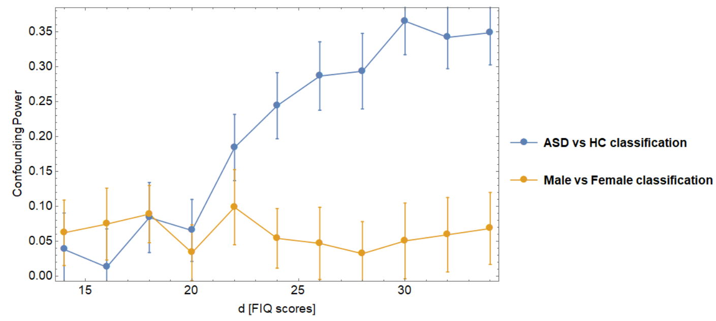
A key aspect of CPX is that it measures the impact of the bias during the classification task under study. Thus, its value represents the relative impact of X in the specific analysis being carried on. For an example of this, see figure 3, in which the value of CPFIQ for the variable Full Intelligence Quotient (FIQ) is reported for a male/female classification task (orange) and for an Autism Spectrum Disorder (ASD) subjects / Healthy Controls (HC) classification task (blue).
COST FUNCTION FOR HIGHLY BIASED DATASETS
An ML algorithm is usually trained to minimize a Mean Squared Loss Function (MSLF), representing the error on the subject class prediction. When the dataset is affected by a bias related to a variable X, a term can be added to MSLF, constraining the training to also maximize the classification error on the subject X label. However, when the bias is strong, this can be counterproductive. To avoid this effect, we developed a cost function that penalizes the errors deriving from a wrong learning pattern related to X. This cost function is: $$MSLF_c=a(output_i,input_i,X_i)∙(output_i-input_i)^2$$
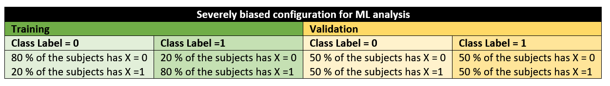
Where inputi ∈{0,1} is the class of the i-th subject, outputi ∈[0,1] represents the classifier estimated probability that the subject belongs to class 1 and a ∈ {1,k} with k>1. Considering the case described in fig. 4, which has a highly biased dataset, the condition for which a=k (as opposed to a=1) is: $$IF (|output_i-input_i|>=0.5\wedge(input_i - X_i)>0)\rightarrow a=k$$
This weights more the errors made when a classification pattern based on the value of X rather than on the class is used. This function has been tested on datasets organized as described in fig. 4.
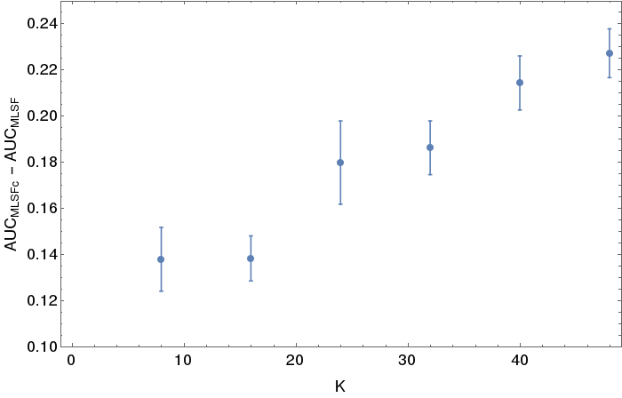
In fig. 5 the results on a male/female classification task are shown as a function of the value of k used in the cost function. The MRI acquisition site was used as confounding variable. Finally, comparing the performances obtained by two networks trained with a traditional MSLF and with MSLFc respectively, it can be observed that, for the first one, 83% of the misclassified subjects belongs to the underrepresented acquisition site, while this accounted for only 54% of the errors of the second network.
CONCLUSION
The proposed index CPx represents a valid instrument for finding confounding variables, while the proposed cost function MSLFc has proved to be successful in minimizing their effects. Despite this study validates this tool in a relatively simple situation, the satisfactory results obtained suggest that extensions of this technique may generalize well.Acknowledgements
No acknowledgement found.References
1. Abraham, Alexandre, et al. "Deriving reproducible biomarkers from multi-site resting-state data: An Autism-based example." NeuroImage 147 (2017): 736-745.
2. Jerome Friedman, Trevor Hastie, and Robert Tibshirani. Sparse inverse covariance estimation with the graphical lasso. Biostatistics, 9(3):432–441, 2008.
3. Han Zhao, Shanghang Zhang, Guanhang Wu, João P Costeira, José MF Moura, and Geoffrey J Gordon. Multiplesource domain adaptation with adversarial training of neural networks. arXiv preprint arXiv:1705.09684, 2017.
4. Di Martino, Adriana, et al. "The autism brain imaging data exchange: towards a large-scale evaluation of the intrinsic brain architecture in autism." Molecular psychiatry 19.6 (2014): 659.
5. Di Martino, Adriana, et al. "Enhancing studies of the connectome in autism using the autism brain imaging data exchange II." Scientific data 4 (2017): 170010.
6. Fischl, Bruce. "FreeSurfer." Neuroimage 62.2 (2012): 774-781.
Figures
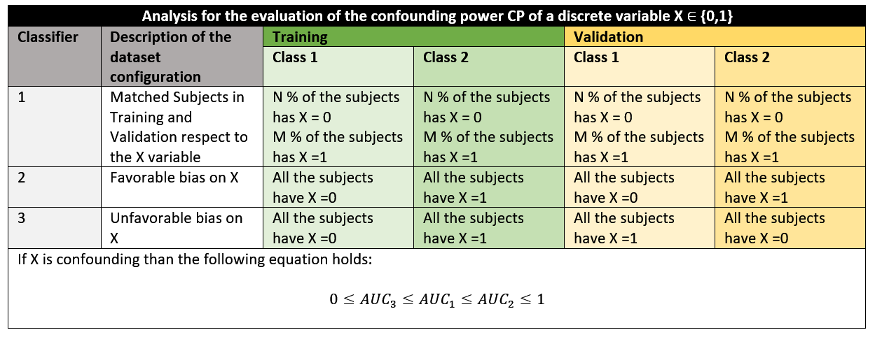
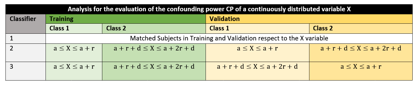
Figure 2: Schematic of the analysis on the confounding power of a continuously distributed variable X. In order to compute the value of CPx for such a variable, it is necessary to discretize its values. This involves two steps:
- Selecting a range of values that represents the discretization step.
- Assessing the confounding power of X, carefully choosing the subjects in the training and validation sets, so that they come from two different discrete intervals. These intervals are characterized by: (1) The distance they have from each other, (2) The starting point of the first unit