4891
Harmonization of Longitudinal MRI Scans in the Presence of Scanner Changes1Electrical and Computer Engineering, Johns Hopkins University, Baltimore, MD, United States, 2Kirby Center for Functional Brain Imaging, Kennedy Krieger Institute, Baltimore, MD, United States, 3Neurology, Johns Hopkins University, Baltimore, MD, United States, 4F.M. Kirby Research Center for Functional Brain Imaging, Kennedy Krieger Institute, Baltimore, MD, United States, 5Radiology and Radiological Sciences, Johns Hopkins University, Baltimore, MD, United States
Synopsis
Longitudinal studies are frequently hampered by changes to scanning protocols, forcing research centers to forgo recommended upgrades to scanning equipment, software, and scan protocol design to allow for consistent scanning. Using a harmonization method that utilizes deep learning and a small (n=12) overlap cohort to learn specific differences between structural MR images before and after a significant scanning change and examined longitudinal data acquired annually over 10 years to determine if bias induced by the scanner change is still present after harmonization. We assessed these results using quantitative metrics for contrast and probed volumetric results using automated segmentation algorithms.
Purpose
Longitudinal studies often rely on quantitative measures to describe the effects of various conditions on their populations. Commonly, volumetric measurements are used to determine how the brain changes over time, for instance to show differences related to age or disease. However, calculation of brain volumes is often left to automated algorithms, which can be biased depending on their input contrasts [1]. In this study, we apply a deep learning-based approach [2] to remove this bias by harmonizing image contrast between before and after a significant change in protocol. To evaluate possible statistical bias due to this procedure, we assessed the effect of this approach on image metrics as well as volume measurements.Methods
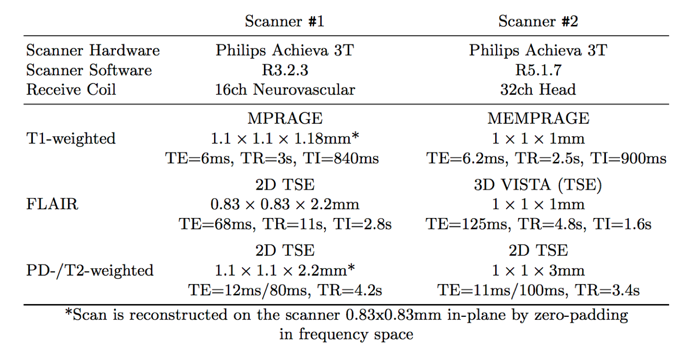
MRI scans for this study were performed under an Institutional Review Board-approved protocol. Subjects for an overlap cohort (n=12, 10 MS patients, 2 healthy controls) were scanned on two scanners (with the appropriate coil and protocol) within 30 days. Scan parameters for both acquisitions are provided in Figure 1. After acquisition, the images were coregistered and the intensities were linearly scaled to align the white matter (WM) peak intensities. The transformation between contrasts was learned through a 2D U-Net modified for synthesis tasks [3]. We further modified this network to reduce the amount of computation required, halving the number of features computed and introducing strided convolutions as a replacement for pooling and upsampling. This allowed for training to be completed in 2 hours for each required network. In addition, a separate network was trained to provide harmonized versions of the Scanner #2 images, even though the contrast did not require matching. This is to allow all harmonized images (from both scanners) to be derived from all input contrasts, reducing random noise that is incoherent between contrasts. To verify this new model, cross-validation of the overlap cohort was conducted, and image similarity metrics were calculated between scanners for both the acquired and harmonized images. To validate longitudinal results, a retrospective analysis of longitudinal data for 25 MS patients collected over 10 years was performed, where each final scan used the Scanner #2 protocol. After preprocessing and harmonization, all images underwent skull removal, white matter lesion (WML) segmentation and whole brain segmentation using an automated pipeline [4-9]. The volume of the cortical grey matter (cGM) was extracted to calculate longitudinal atrophy. In addition, coefficient of variation (CoV) of WM and cGM and specific contrast (WM to cGM, WM to CSF and WM to WML) were calculated as quantitative surrogates of contrast using automated segmentation results. Statistical significance was derived using a linear mixed effects model for longitudinal measures and a Wilcoxon signed-rank test for all paired measurements (α=0.01).Results/Discussion
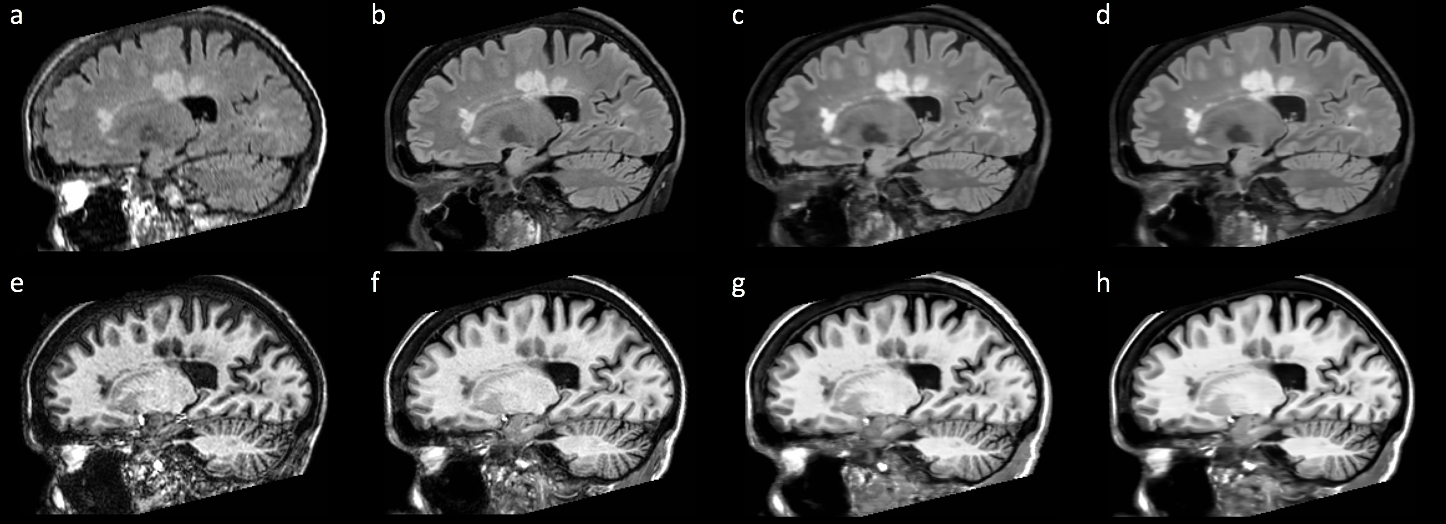
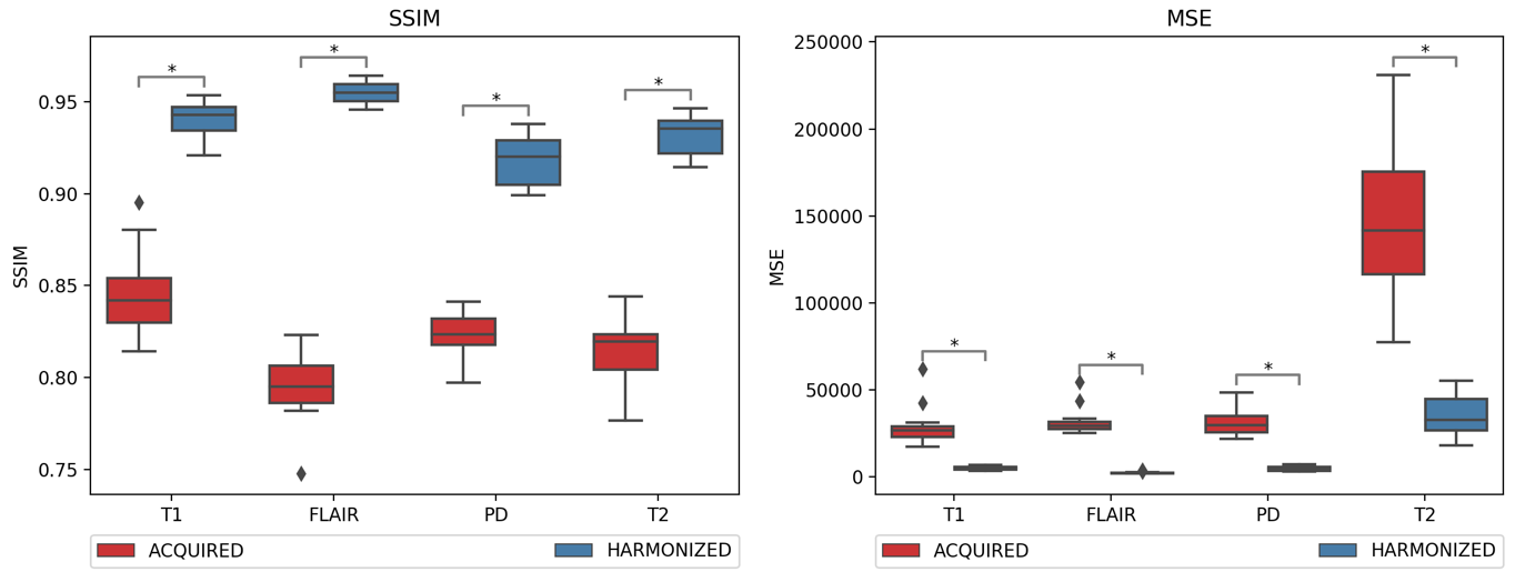
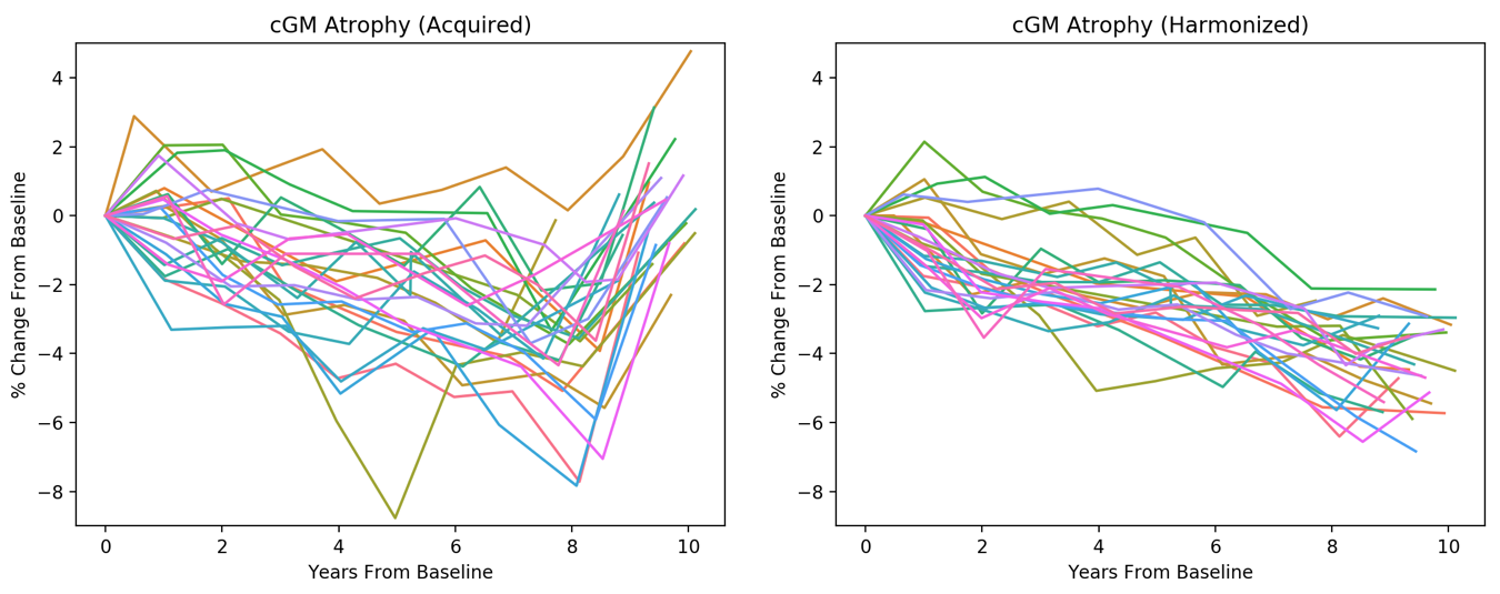
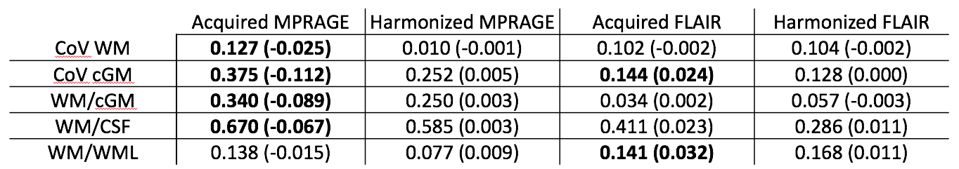
Figure 2 depicts representative slices of the process for the FLAIR and T1-weighted contrasts before and after harmonization. These images show substantially improved similarity between the images, which is quantified in the image similarity metrics for the overlap cohort in Figure 3. We can see that the slimmer network still shows significant, substantial improvement in all contrasts for both similarity metrics. In Figure 4, we see that in the acquired trajectories, each patient has a significant increase in cGM volume at their last scans (acquired on Scanner #2). This is greatly reduced and no longer a significant change when using the harmonized images. A linear mixed effects model using clinical covariates such as age and sex was also significantly more accurate in predicting change in cGM when using harmonized images. Finally, Figure 5 outlines the differences observed in the quantitative measures of contrast. We can see a significant difference in CoV for both cGM and WM for the T1-weighted images, as well as in the cGM of the FLAIR images. In the contrast measures, there was significant difference in WM to cGM and WM to CSF contrast in the acquired T1-weighted images and in the WM to WML the acquired FLAIR images. These differences are substantially reduced and no longer significant in the harmonized images.Conclusions
In this longitudinal analysis of deep learning-based harmonization, we find that significant biases in volumetric results derived from a change in scanner/protocol are removed and differences are substantially reduced. The harmonized images are also significantly more similar when compared using image comparison metrics and in a quantitative comparison of contrast. This has important potential for longitudinal studies, allowing to upgrade scanner equipment and imaging protocols and removing contrast changes due to such updates through the acquisition of data for a small overlap cohort and implementation of harmonization as a preprocessing step in automated analysis.Acknowledgements
Research funded by NIH R01NS082347, NIH P41 EB015909, and the National MS Society (TR, RG-1601-07180).References
[1] Biberacher,V.,Schmidt,P.,Keshavan,A.,Boucard,C.C.,Righart,R.,Sämann,P.,Preibisch,C., Fröbel, D., Aly, L., Hemmer, B., Zimmer, C., Henry, R.G., Mühlau, M.: Intra-and interscanner variability of magnetic resonance imaging based volumetry in multiple sclerosis. NeuroImage 142, 188–197 (2016)
[2] Dewey, B.E., Zhao, C., Carass, A., Oh, J., Calabresi, P.A., van Zijl P.C.M, Prince, J.L.: Deep Harmonization of Inconsistent MR Data for Consistent Volume Segmentation. In: A. Gooya et al. (Eds.): SASHIMI 2018. LNCS, vol. 11037. Springer (2018)
[3] Zhao, C., Carass, A., Lee, J., He, Y., Prince, J.L.: Whole Brain Segmentation and Labeling from CT Using Synthetic MR Images. In: Machine Learning in Medical Imaging. pp. 291–298. Springer International Publishing (2017)
[4] Roy, S., Butman, J. A., Pham, D. L., Alzheimers Disease Neuroimaging Initiative. (2017). Robust skull stripping using multiple MR image contrasts insensitive to pathology. Neuroimage, 146, 132–147. http://doi.org/10.1016/j.neuroimage.2016.11.017
[5] Huo, Y., Plassard, A. J., Carass, A., Resnick, S. M., Pham, D. L., Prince, J. L., & Landman, B. A. (2016). Consistent cortical reconstruction and multi-atlas brain segmentation. Neuroimage, 138, 197–210. http://doi.org/10.1016/j.neuroimage.2016.05.030
[6] Roy, S., He, Q., Sweeney, E., Carass, A., Reich, D. S., Prince, J. L., & Pham, D. L. (2015). Subject-Specific Sparse Dictionary Learning for Atlas-Based Brain MRI Segmentation. IEEE Journal of Biomedical and Health Informatics, 19(5), 1598–1609. http://doi.org/10.1109/JBHI.2015.2439242
[7] Dewey et al. Automated, Modular MRI Processing for Multiple Sclerosis using the BRAINMAP Framework. ECTRIMS Online Library. October 26, 2017
[8] Avants, B. B., Tustison, N. J., Song, G., Cook, P. A., Klein, A., & Gee, J. C. (2011). A reproducible evaluation of ANTs similarity metric performance in brain image registration. Neuroimage, 54(3), 2033–2044. http://doi.org/10.1016/j.neuroimage.2010.09.025
[9] Wang,H., Suh,J.W., Das,S.R, Pluta,J., Craige,C., Yushkevich,P.A.: Multi-Atlas Segmentation with Joint Label Fusion. IEEE Transactions on Pattern Analysis and Machine Intelligence 35(3), 611–623 (Mar 2013)
Figures