4886
Analyzing multi-exponential T2 decay data using a neural network1Physics & Astronomy, University of British Columbia, Vancouver, BC, Canada, 2International Collaboration on Repair Discoveries, Vancouver, BC, Canada, 3Biomedical Engineering, University of British Columbia, Vancouver, BC, Canada, 4Radiology, University of British Columbia, Vancouver, BC, Canada, 5Kinesiology, University of British Columbia, Vancouver, BC, Canada, 6Pathology & Laboratory Medicine, University of British Columbia, Vancouver, BC, Canada
Synopsis
The water molecules within a single voxel may exist in different microenvironments so that the T2 relaxation is considered as a multi-exponential decay. A few quantitative imaging techniques such as myelin water imaging attempt to extract the short T2 component as a marker specific to myelin. However, decomposition of multi-exponential T2 decay data is an ill-posing problem. Commonly used non-negative least squares fitting method is slow, complex and unstable, even with strong regularization and B1 correction. We used synthetic data to train a single neural network for a better and faster analysis of the multi-exponential T2 decay data.
Introduction
T2 relaxation in brain and spinal cord white matter is governed by the microenvironment of water molecules. Myelin water, the water trapped in myelin bilayers, exhibits shorter T2 than that of the intra/extra (IE) cellular water. The T2 relaxation curve of each voxel in the white matter is thus considered a multi-exponential decay.1 Decomposition of such multi-exponential T2 decay curve data is a complex and often unstable process. Non-negative least squares (NNLS) is a commonly used technique which can fit voxel-wise T2 decay data to create a T2 distribution, from which the myelin water fraction (MWF, the ratio of myelin water signal to the total signal), mean T2 of myelin water (MWT2), and mean T2 of IE water (IEWT2) can be extracted.1,2 The latest NNLS analysis incorporates the extended phase graph (EPG) algorithm to estimate the refocusing flip angle (FA) of each voxel to correct for the effect of stimulated echoes.3 However, NNLS analysis is slow due to its complexity and strong regularization for stability.
Machine learning approaches may provide an alternative to NNLS analysis of multi-exponential T2 decay data. We previously used synthetic data to train four different neural networks to estimate MWF, MWT2, IEWT2, and FA individually.4 Our objective for this study was to develop a single neural network that is capable of performing multi-exponential T2 decay data analysis to estimate MWF, MWT2, IEWT2, and FA simultaneously.
Methods
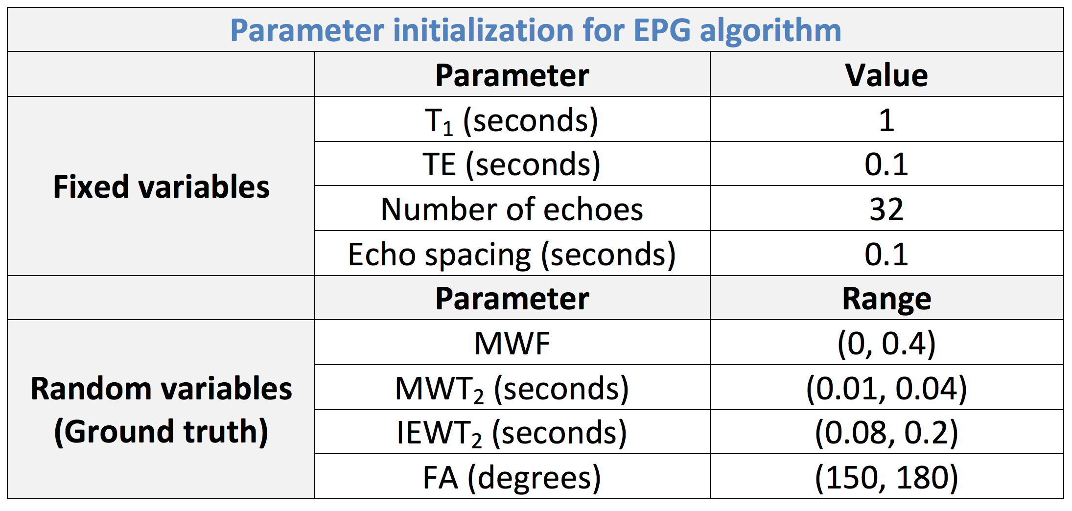
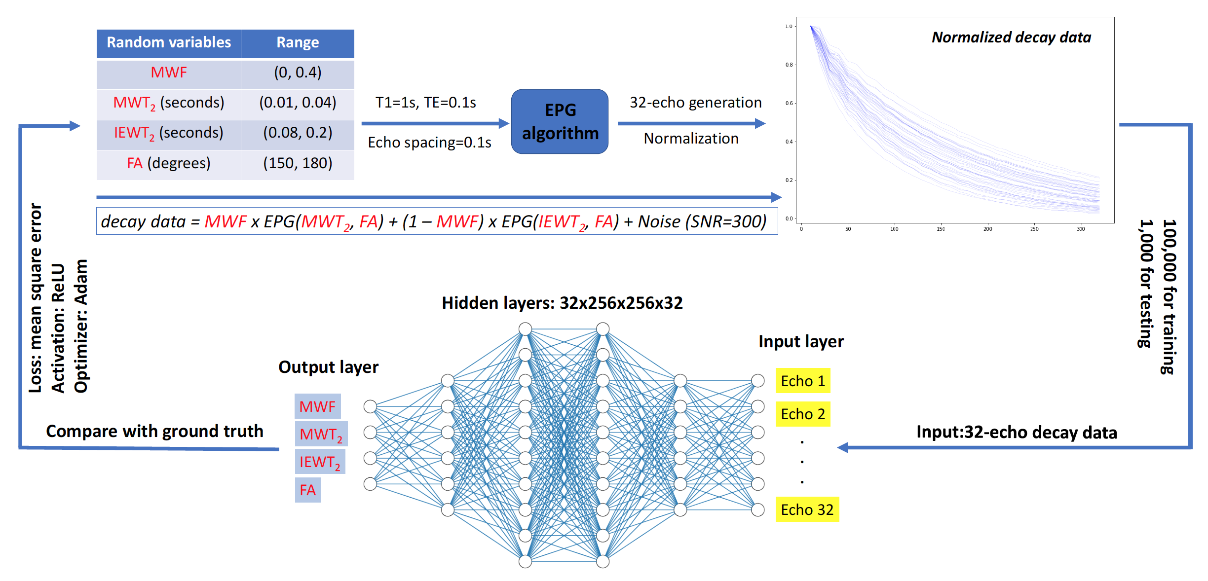
MR data simulation: 32-echo T2 decay data for a two-pool model (myelin water and IE water) were simulated by EPG algorithm.5 All EPG parameters were initialized according to Table 1 and the decay data were synthesized as decay data = MWF x EPG(MWT2, FA) + (1–MWF) x EPG(IEWT2, FA) + Noise(SNR=300). The decay data were subsequently normalized to set the first echo as unity. 100,000 synthesized 32-echo decay curves were generated for training and 1,000 for testing. Training and testing data were generated and stored independently.
Neural network models: A single neural network with 6 fully connected layers (32×32×256×256×32×4) was constructed (activation function: ReLU, optimizer: Adam6, loss: mean square error) to solve for MWF, MWT2, IEWT2, and FA simultaneously. Figure 1 depicts the schematic of data synthesis and network training.
Trained model and NNLS calculation: The generated 1,000 synthesized 32-echo decay testing data were analyzed by the neural network model and NNLS (in-house software) independently to simultaneously determine MWF, MWT2, IEWT2, and FA for each decay curve.
Results & Discussion
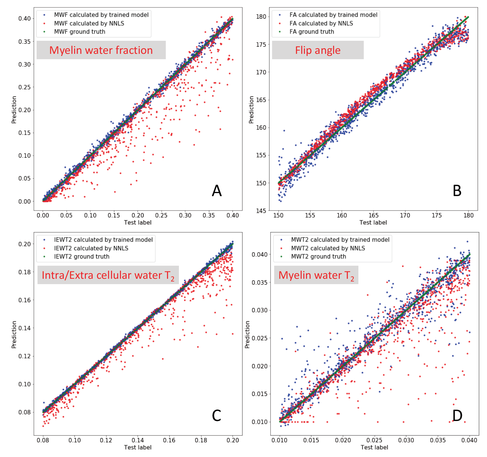
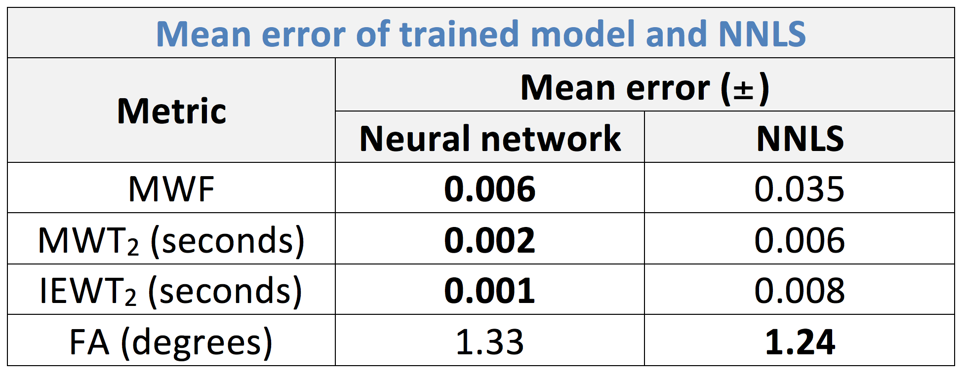
The neural network model results are plotted against the ground truth labels in Figure 2. The mean errors of both methods are presented in Table 2. In the predictions of MWF (Figure 2(A)) and IEWT2 (Figure 2(C)), the trained model demonstrated much better agreement with the ground truth than NNLS. The scatter of the points by NNLS calculation illustrates the instability of NNLS and systematical underestimation of MWF and IEWT2. For the estimation of FA (Figure 2(B)), both methods performed at a high level of accuracy. Unfortunately, neither of the two methods worked well in the calculation of MWT2 (Figure 2(D)). However, further training and fine-tuning may improve the performance of the neural network model.
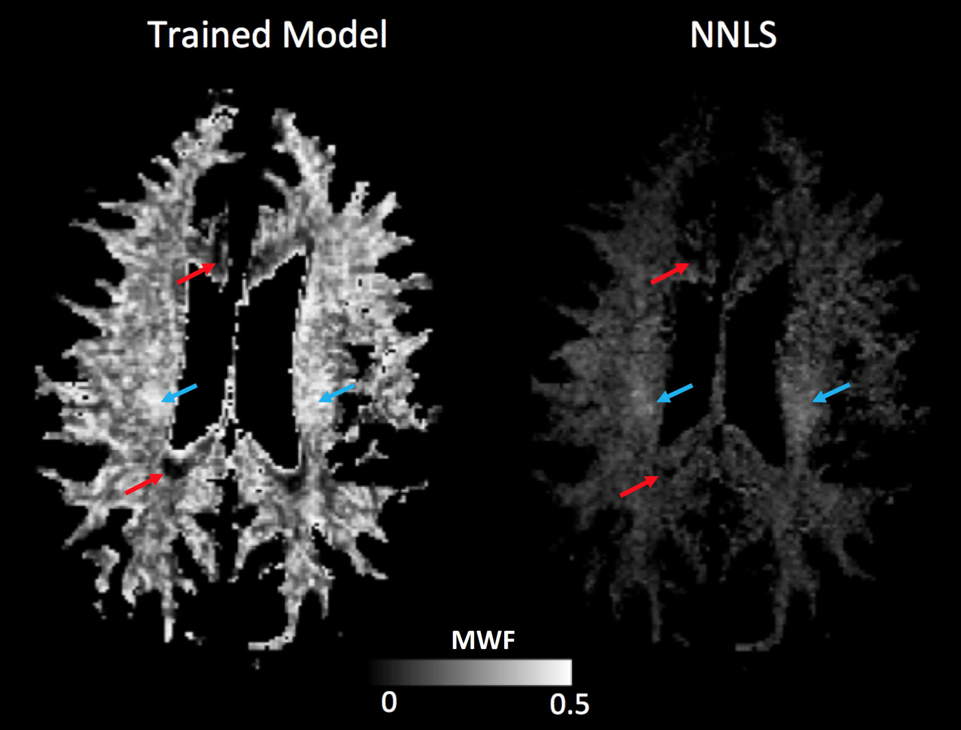
We also applied the neural network model to one example of in-vivo MWI data (32 echo, TE/TR=10/1000ms) and compared the resulting MWF with NNLS (Figure 3). Although the neural network model reports much higher overall average MWF (0.279) than NNLS (0.082), some similar features between the two MWF maps were observed (Figure 3, arrows). Lower in-vivo MWF estimated by NNLS was consistent with the underestimation problem that we observed in the simulation study. The neural network model is also undermined by the fact that the training data generated by a two-pool simulation may not be a good representation of in-vivo data, possibly causing MWF overestimation. Since there is no ground truth available for the in-vivo data, it’s difficult to assess the accuracy of the two methods definitively. Nevertheless, it only takes approximately 20s for the neural network model to perform whole brain analysis while NNLS needs at least 1.5 hours using MATLAB on a CPU processor with 6 cores (3.50GHz).
Conclusion
In this simulation study, a single trained neural network model with multi-output architecture outperforms the conventional NNLS algorithm in both accuracy and processing speed when analyzing synthetic multi-exponential T2 decay data. Large differences in mean MWF were observed in the analysis results of in-vivo data by these two methods. In the future, we will generate training and testing data using a many-pool simulation to improve the current model.Acknowledgements
We thank the study participants and the excellent MRI technologists at the UBC MRI Research Centre. Funding support was provided by the Multiple Sclerosis Society of Canada, Natural Sciences and Engineering Research Council Discovery Grant.References
1. Whittall KP, MacKay AL. Quantitative interpretation of NMR relaxation data. Journal of Magnetic Resonance (1969). 1989;84(1):134-152.
2. MacKay A, Whittall K, Adler J, Li D, Paty D, Graeb D. In vivo visualization of myelin water in brain by magnetic resonance. Magn Reson Med. 1994;31(6):673-677.
3. Prasloski T, Mädler B, Xiang Q, MacKay A, Jones C. Applications of stimulated echo correction to multicomponent T2 analysis. Magnetic Resonance in Medicine. 2012;67(6):1803-1814.
4. Liu H, Tam R, Kramer J, Laule C. Myelin water imaging data post-processing: A deep learning approach. Proc. Into. Soc. Mag. Reson. Med, Machine Learning Workshop Part II, 2018.
5. Hennig J. Multiecho imaging sequences with low refocusing flip angles. Journal of Magnetic Resonance. 1988;78(3):397-407.
6. Kingma DP, Ba J. Adam: A method for stochastic optimizaton. arXiv. 2014;1412.6980.
Figures