4874
Deep Predictive Modeling of Dynamic Contrast-Enhanced MRI Data1Electrical Engineering, Stanford University, Stanford, CA, United States, 2Radiology, Stanford University, Stanford, CA, United States
Synopsis
This work demonstrates the use of recurrent generative spatiotemporal autoencoders to predict up to fifteen future frames of abdominal DCE-MRI video data, starting with only three ground truth input frames for context. The objective is to predict what healthy patient video data and organ-specific contrast curves look like, to expedite anomaly detection and enable pulse sequence optimization. The model in this study shows promise; it was able to learn contrast changes without losing structural resolution during training time, and lays the foundation for future work.
Introduction
Dynamic contrast-enhanced MRI (DCE-MRI) provides an effective non-invasive assessment of the kidneys, livers, and other organs, and is particularly useful for oncological diagnosis. Two key challenges that diminish the clinical effectiveness of DCE-MRI are: the difficulty of optimizing for both spatial and temporal resolution, as well as local anatomy-of-interest resolution, due to already long scan times, and the lengthy manual data processing to quantify tissue perfusion and identify potential anomalies. Building on existing video prediction work,1,2 we propose to use a recurrent generative spatiotemporal autoencoder model to predict contrast enhancement curves from initial pre-contrast images. By learning the contrast curves, the model enables real-time pulse sequence adjustments to optimize signal and contrast at key times and locations. Additionally, if the network can predict healthy behavior, the actual data can be compared with the prediction to quickly identify anomalies and compare tissue perfusion rates.Methods
Four-dimensional data from 100 patient volunteers are used; 70 patients for training, 10 for validation, and 20 for testing. Data was acquired using a T1-weighted, 3D spoiled gradient recalled (SPGR) sequence on a GE 3T MR750 scanner, with a 32-channel cardiac coil.3 Several preprocessing steps are taken: slices are zero-padded in the x- and y-directions so all images are the same dimensions, and the data is normalized. For initial proof of concept, only image magnitude is used. The first three ground truth frames are concatenated along the channel dimension for the first input. During training time, additional ground truth frames are used to predict each timestep. During validation time, predictions are concatenated to make the next predictions.
The autoencoder architecture is shown in Figure 1. The objective of the encoder is to embed the key features of the inputs, from which the decoder produces the next time frame. The encoder is based on a VGG16 model without fully-connected layers at the end.4 The decoder upsamples and deconvolves, and adds a residual skip connection from the previous corresponding layers during the encoding network to assist with learning structural similarities. The loss function is a weighted mean squared error (MSE), with a higher weighting on the earlier frame predictions. In TensorFlow, we use the Adam optimizer to minimize dependence on learning rate tuning.
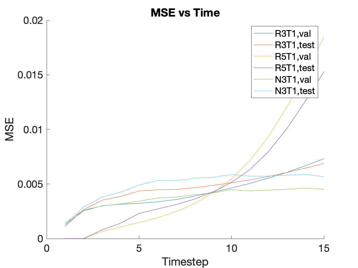
The three primary models are: a recurrent three-to-one (R3T1) model, a recurrent five-to-one (R5T1) model, and a non-recurrent three-to-one (N3T1) model. The R3T1 model is modelled after typical recurrent neural network (RNN) architectures, where the encoder and decoder share weights from timestep to timestep. The R5T1 model is an experiment to evaluate the benefits of more context frames. The N3T1 model is an unrolled model, which trains independent weights per timestep, which should theoretically improve performance at the cost of increased weights.
Results & Discussion
Figure 2 shows the training results in sets of 3. The top set is from the R3T1 model, the middle set is the R5T1 model, and the bottom set is the N3T1 model. In each set, the top row is the ground truth frames, the middle row is the predicted frames, and the bottom row is the difference. All three models appear to perform well during training. Figure 3 shows the validation results for two slices over time. From left to right are the ground truth, R3T1 model, R5T1 model, and N3T1 model predictions. The early predictions are similar to the ground truth frames, but cases where one prediction diverges drastically from the ground truth, the following predicted frames deviate increasingly. This conclusion is evident in Figures 4 and 5. Figure 4 is the contrast enhancement curve, specifically for the liver. Figure 5 is the plot of MSE over time. The N3T1 model demonstrates the best performance over time as expected since each timestep trains unique weights. In practice, the predictive model will be combined with the data acquisition process and update the prediction as real data is acquired, so performance is expected to improve for all models.Conclusion
The evaluated models demonstrate the ability of a deep predictive model to learn contrast changes in abdominal DCE-MRI data. Different models are presented, each using time and context information differently, but ultimately drawing a similar conclusion: accurate prediction of each timestep is crucial to ensure no deviations that impair future predictions. One limitation with this study is that the data available to us came from patients with an assortment of abnormalities, since healthy pediatric patients are not often scanned. We believe, though, that training this network would only improve in accuracy if trained on healthy patient data, since there would be more anatomical consistency across patients.Acknowledgements
This work was generously supported by NIH R01-EB009690, NIH R01-EB026136, and GE Healthcare.References
- Feng X, Meyer C. Accelerating cardiac dynamic imaging with video prediction using deep predictive coding networks. ISMRM. 2018.
- Srivastava N, Mansimov E, Salakhutdinov R. Unsupervised learning of video representations using LSTMs. Proceedings of International Conference on Machine Learning (ICML). 2015.
- Zhang T, Cheng JY, Potnick AG, et al. Fast pediatric 3D free-breathing abdominal dynamic contrast-enhanced MRI with high spatiotemporal resolution. J Magn Reson Imaging. 2015;41:460-473.
- Simonyan K, Zisserman A. Very deep convolutional networks for large-scale image recognition. arXiv:1409.1556 [cs.LG]. 2015.
Figures
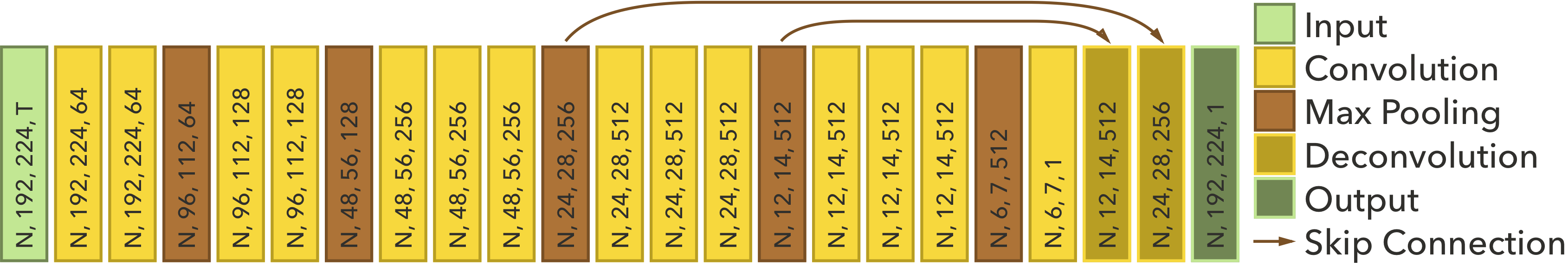
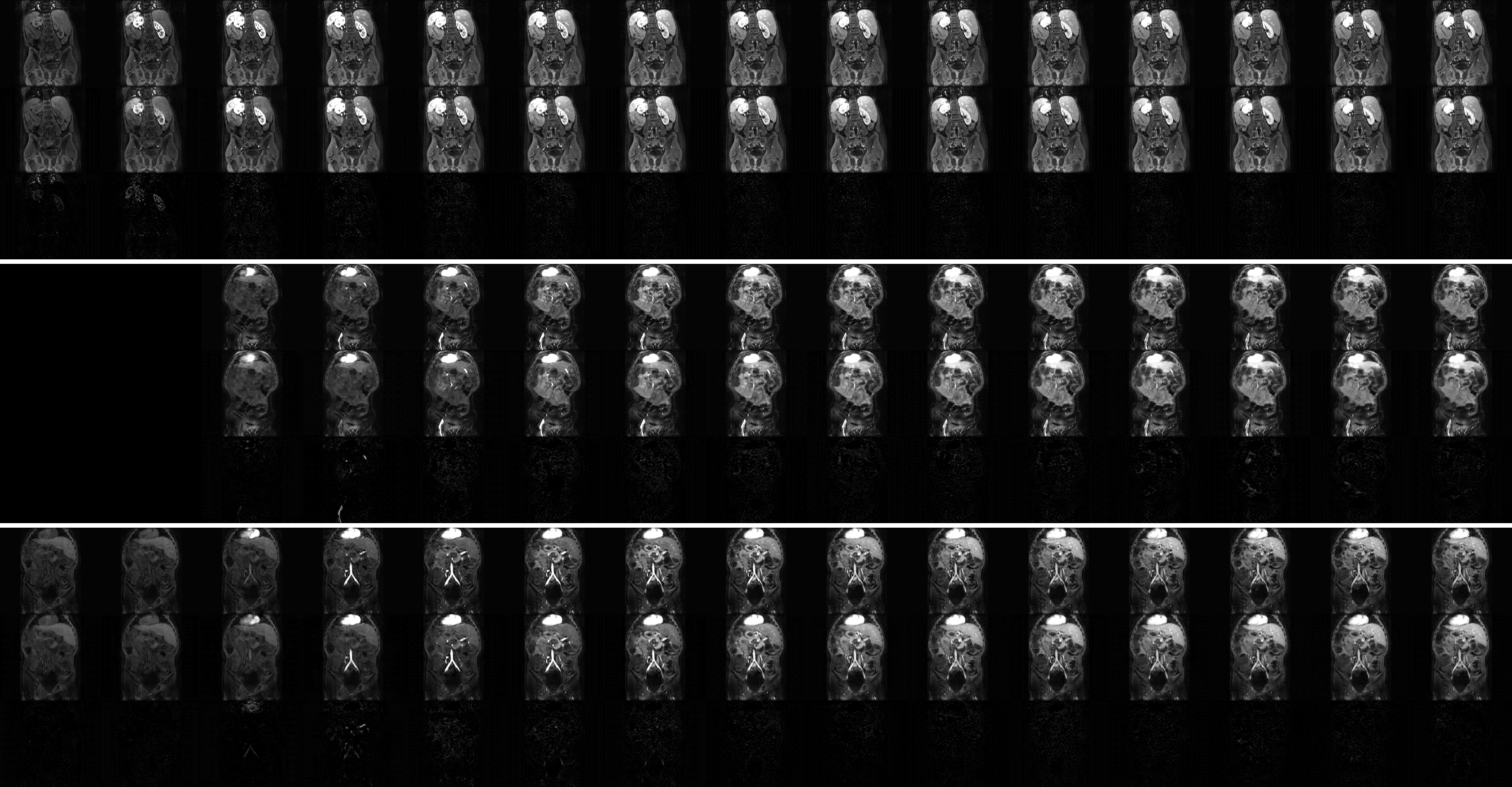
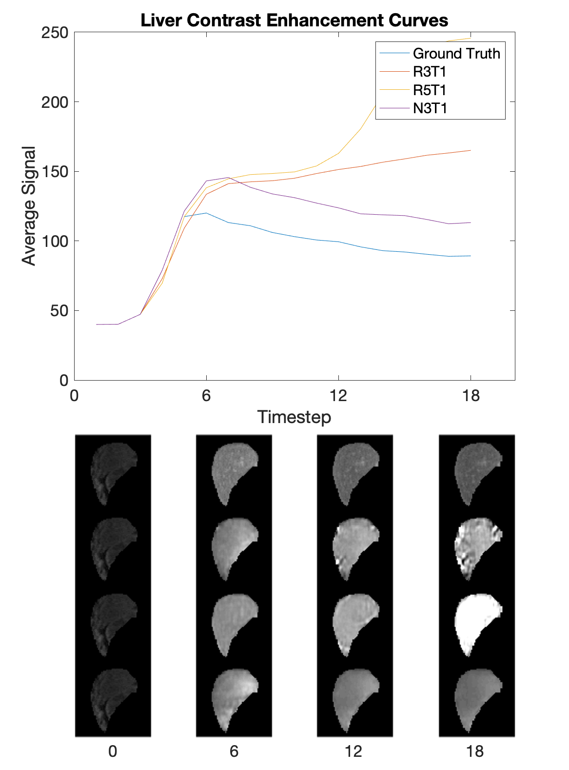
Figure 4. The contrast enhancement curve for the liver, with selected, segmented timesteps shown. The liver was manually segmented and the average signal was calculated at each timestep. Qualitatively, the shape of the curve for N3T1 looks best, albeit offset by a constant value.