4866
Visualizing the “ideal” input MRI for synthetic CT generation with a trained deep convolutional neural network: Can we improve the inputs for deep learning models?1University of California San Francisco, San Francisco, CA, United States, 2UC Berkeley - UC San Francisco Joint Graduate Program in Bioengineering, Berkeley and San Francisco, CA, United States
Synopsis
Deep learning has found wide application in medical image reconstruction, transformation, and analysis tasks. Unlike typical machine learning workflows, MRI researchers are able to change the characteristics of images that are used as inputs to deep learning models. We proposed an algorithm that allows us to visualize the “ideal” input images that would provide the least error for a trained deep neural network. We apply this visualization technique on a deep convolutional neural network that converts Dixon MRI to synthetic CT images. We briefly characterize the optimization behavior and qualitatively analyze the features of the “ideal” input image.
Introduction
Deep neural networks have found large use in medical imaging on different applications: image segmentation, lesion detection, image reconstruction, image modality transformation, etc. Typically, machine learning practitioners only have control over the models that they use for supervised learning: the input data and labels are pre-defined and fixed. However, magnetic resonance imaging scientists have a large degree of control over the images that are used as inputs to deep learning models.
Researchers can visualize the behavior of image classification deep neural networks through the use of saliency maps1. The limitation of these saliency maps is that they are only applicable to classification networks. These cannot be directly applied to networks that have an image as an output since saliency maps are computed based on derivatives of the output score (scalar) with respect to the input pixels. Directly applying saliency maps to image outputs means computing a derivative for every output pixel, and specific output pixels in themselves do not determine accuracy in prediction.
In this abstract, we propose an optimization-based method to solve for the ideal inputs to a trained neural network for a particular target output; this is analogous to the maximum-class-activation saliency map but for an image output. We examine a deep convolutional neural network that generates a synthetic CT image from Dixon MRI input2. We qualitatively describe the features of the ideal MRI to potentially tune the image acquisition.
Methodology
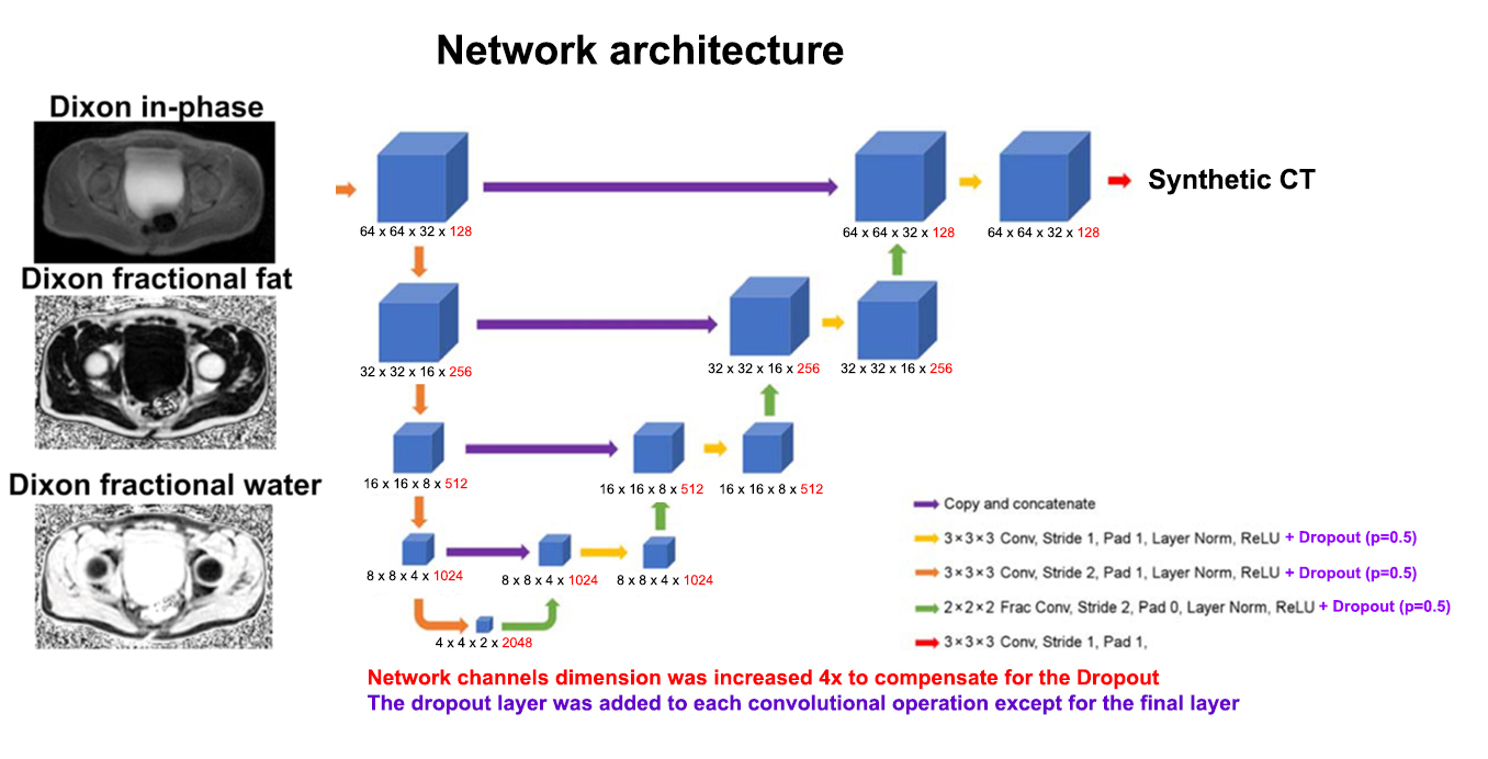
A deep convolutional neural network for generating synthetic CT images from Dixon in-phase, Dixon fractional fat, and Dixon fractional water images was used2. The network architecture is shown in Figure 1.
In the class model visualization procedure for an image classification model1, the optimization objective was:
$$\underset{I}{\arg\max} \space S_c(I) + \lambda ||I||_2^2$$ (eq. 1)
where
$$S_c(I) = f(I; \bar\omega)$$
and $$$f$$$ is the trained deep neural network and $$$\bar\omega$$$ are the parameters of the trained network.
We restate this for an image output as:
$$\underset{I}{\arg\max} \space ||f(I; \bar\omega)-y||_1 +\lambda_1 ||\text{ReLU}(I-1.0)||_2^2+\lambda_2||\text{ReLU}(-I)||_2^2$$ (eq. 2)
where $$$\bar\omega$$$ are the parameters of the trained deep neural network shown in Figure 1, and is the target ground-truth CT image patch. In other words, we solve for the input image $$$I$$$ for the deep convolutional neural network $$$f$$$ that matches the ground-truth CT image patch $$$f$$$ as closely as possible. The additional terms penalize input image values outside the range 0.0 to 1.0.
We solved the optimization problem above (eq. 2) using the L-BFGS optimization algorithm (learning rate=1.0, max. iterations=20, number of gradient steps=100) and was implemented in PyTorch (v.0.4.1). We investigated the effect of different image initializations on the optimization: (1) a random uniform noise image with range 0.0 to 1.0, (2) a uniform image with all zeros, and (3) the corresponding patient Dixon MRI. Furthermore, we analyze the qualitative features of the calculated optimal input.
Results
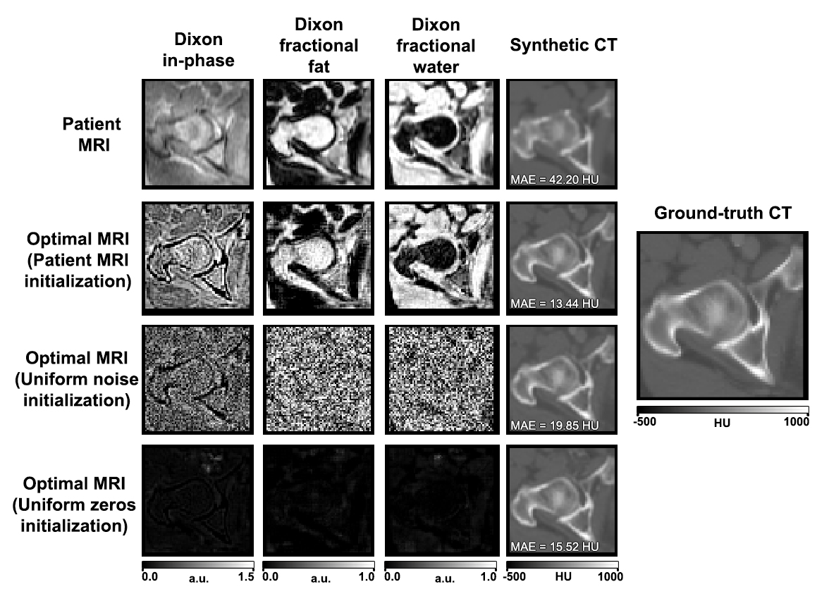
Figure 2 shows the effect of initialization to the computed optimal input image. Since the network is non-linear, the optimization has several local minima that produce a good synthetic CT image. Uniform noise initialization appears to produce Dixon fractional fat and fractional water images that still appear to be noise, but produce good synthetic CT images. Initialization with a uniform image with all zeros produces MRI with very low image intensities. Since we are interested in improving the MRI acquisition parameters, we further analyze images initialized from patient MRI.
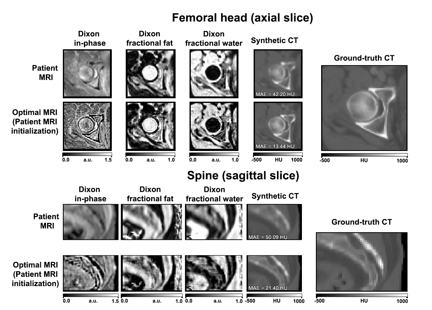
Figure 3 shows the optimal MRI images around the femoral head and spine. We observe that the Dixon fractional fat and fractional water images between patient MRI and optimal MRI look very similar. However, the Dixon in-phase of the optimal MRI is much sharper suggesting that bone needs to be enhanced in the patient MRI acquisition to improve synthetic CT generation.
Discussion and Conclusion
We developed an approach to visualize the “ideal” input image for deep neural networks with image outputs by restating an image classification model visualization technique. We explored this visualization technique for a CNN that estimates synthetic CT images from a set of Dixon MRI images. We successfully generated “ideal” input images for a particular target image. For this application, we found that in order for the network to generate better synthetic CT images, cortical bone in the Dixon in-phase image needs to be more defined. This suggests either increasing the spatial resolution, decreasing spatial blurring and chemical shift artifacts, or using a sequence that enhance edges in regions of thin cortical bone. This approach can be broadly applied to deep neural networks with image outputs, and provides a new mechanism for optimization of inputs in these problems.Acknowledgements
This work was supported by an NVIDIA GPU grant and NIH grant R01CA212148.References
[1] K. Simonyan, A. Vedaldi, and A. Zisserman, “Deep Inside Convolutional Networks: Visualising Image Classification Models and Saliency Maps,” arXiv:1312.6034 [cs], Dec. 2013.
[2] A. P. Leynes and P. E. Z. Larson, “Synthetic CT Generation Using MRI with Deep Learning: How Does the Selection of Input Images Affect the Resulting Synthetic CT?,” in 2018 IEEE International Conference on Acoustics, Speech and Signal Processing (ICASSP), 2018, pp. 6692–6696.
Figures