4865
The impact of variable MRI acquisition parameters on deep learning-based synthetic CT generation1Image Sciences Institute, University Medical Center Utrecht, Utrecht, Netherlands, 2Department of Orthopedics, University Medical Center Utrecht, Utrecht, Netherlands, 3MRIguidance, Utrecht, Netherlands
Synopsis
Deep learning-based synthetic CT generation models are generally trained and evaluated on MR images obtained with a single set of acquisition parameters. In this study, we investigated the robustness of such models to clinically plausible changes in acquisition parameters by training and evaluating models on MR images acquired and reconstructed from gradient echo sequences at different echotimes (TE), resolution and flip angles. We investigated the sensitivity to TEs by training models on randomly interspersed multi-echo gradient echo MR images acquired at different TEs. Multi-echo trained models achieved better generalization performance to varying acquisition parameters without excessively compromising results on dedicated data.
Introduction
In the last decade, deep learning (DL) based synthetic CT (sCT) generation has shown promising benefits in terms of workflow efficiency in radiotherapy treatment planning1 and for orthopedic clinical practice. However, in most DL studies, models are trained and evaluated on data obtained from the same scanners, with the same sequence and acquisition parameters. This may prevent widespread adoption, as different centers have different hardware (e.g. different gradient systems) leading to variable acquisition parameters in terms of echo and repetition times, flip angles and resolution, resulting in different contrast weightings. In this study, we investigated how clinically plausible variations in MR acquisition parameters impact sCT generation by training and evaluating DL models on MR images with different echo times (TE).
Methods
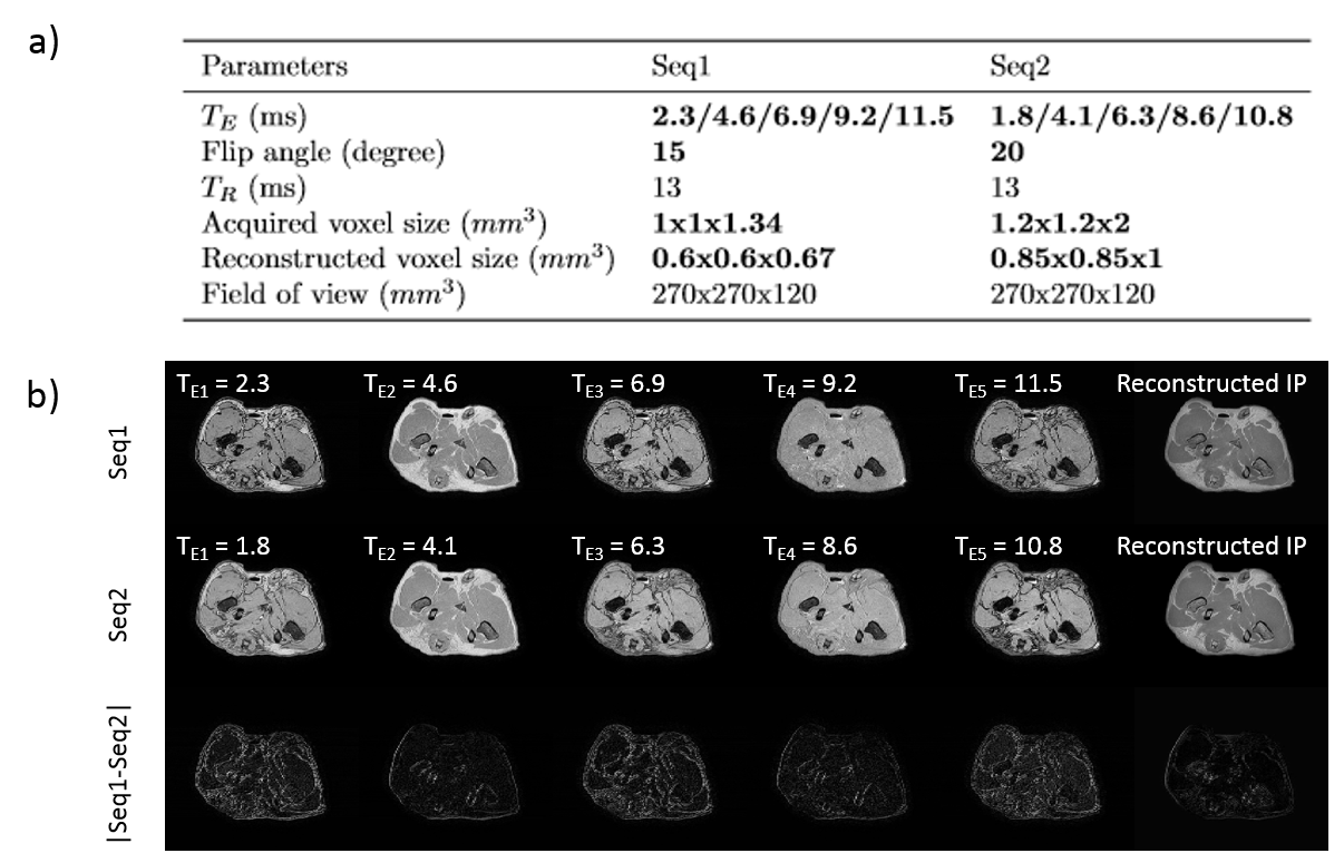
Acquisition An ex vivo study was performed on 17 domestic dogs deceased of natural causes which underwent CT (Brilliance CT big bore, Philips) and MR (1.5T, Ingenia, Philips Healthcare, Best, Netherlands) imaging for scientific purposes. MR images were acquired using two three-dimensional radio-frequency spoiled T1-weighted multiple gradient echo mDixon2,3 sequences with slightly different acquisition parameters as presented in Figure 1-a. They consist of five acquired echoes and in-phase (IP), water (W) and fat (F) reconstructions as presented Figure 1-b. The i-th echo of the sequences 1 and 2 will be referred to as Seq1-TEi and Seq2-TEi. CT slice spacing was 0.7 mm and pixel spacing ranged between 0.4/0.8 mm.
Image pre-processing CT data was non-rigidly registered to the second echo of each sequence (Elastix4) and all images were resampled to 0.85x0.85x1 mm3.
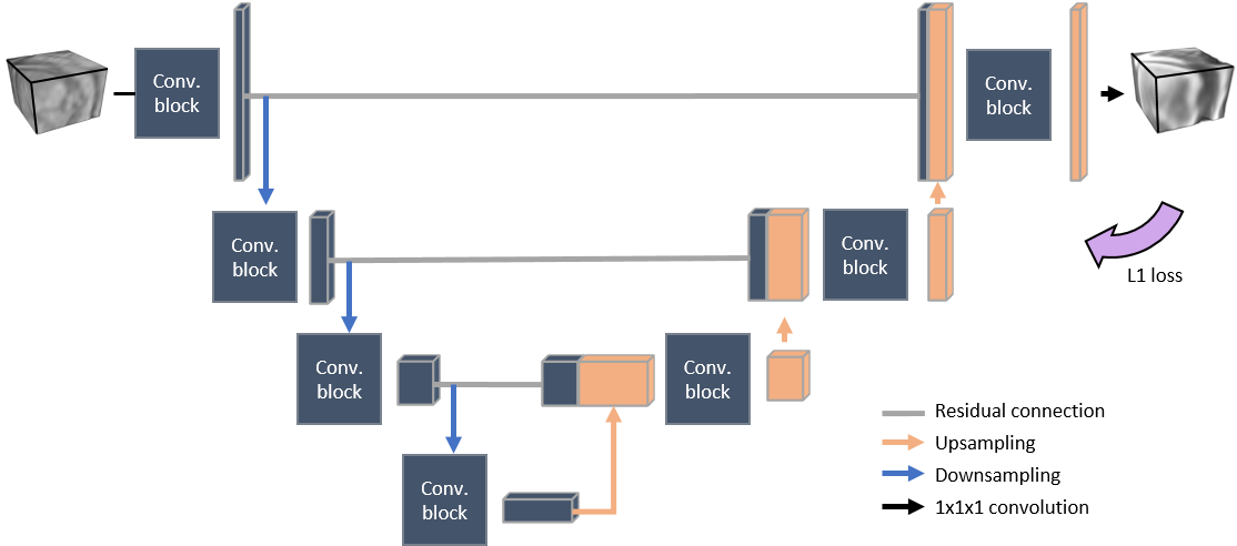
sCT generation A paired 3D patch-based UNet represented in Figure 2 was trained to learn a mapping from MR intensities to CT Hounsfield units (HU). All trainings were performed on images from Seq1 to investigate the transferability of such models to Seq2-TE2 (almost IP). Five models were trained, either on a single TE (Seq1-TE2 (acquired IP) or reconstructed Seq1-IP) or on multiple TEs randomly interspersed during the training phase (TE-augmentation). Combinations we used for TE-augmentation were TE1 & TE2, TE2 & TE4 or all echoes together. For each of these five models trained on Seq1, evaluations were performed on:
- Seq2-TE2 to investigate model transferability from Seq1 to Seq2;
- simulated images (STE) computed from sequence 1 (Seq1-STE) to investigate the sensitivity of the prediction to TE;
- Seq1-TE2 to investigate the effect of TE-augmentation compared to a model specifically trained on Seq1-TE2.
Evaluations were performed on TE2 as it is the first IP echo which presumably has the best contrast for sCT generation. Seq1-STE were generated from Seq1 W and F images using a multi-peak fat model using $$$ S_{T_E}=|W+F\times f_{T_E}| $$$ and $$$f_{T_E}=\sum_{\text{fat peaks}}\alpha_p\exp(2i\pi\times f_F \times\gamma B_0\times T_E)$$$ where $$$\alpha _p$$$ and $$$f_F$$$ are the relative amplitude (%) and frequencies (ppm) of the fat H-NMR signal as reported by Hamilton et al.5.
sCTs were generated for all subjects using a three-fold cross-validation with 12/6 subjects in the training/testing sets. The same subject was never present in both sets. The evaluation comprises mean absolute error (MAEbody) computed within the body contour and MAEbone and Dice similarity coefficient (DSCbone) computed within bone masks (CT HU > 200).
Results
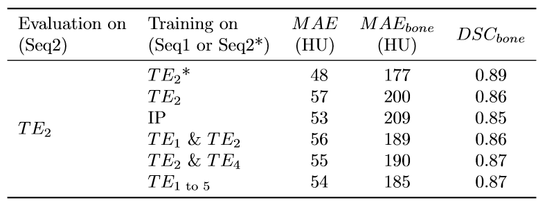
Figure 3 shows that transferring a model from Seq1-TE2 to Seq2-TE2 resulted in higher errors than applying a model specifically trained on Seq2-TE2. When evaluated on Seq2-TE2, models trained on Seq1 using TE-augmentation outperformed models trained on most similar TEs from Seq1 (acquired Seq1-TE2 and reconstructed Seq1-IP).
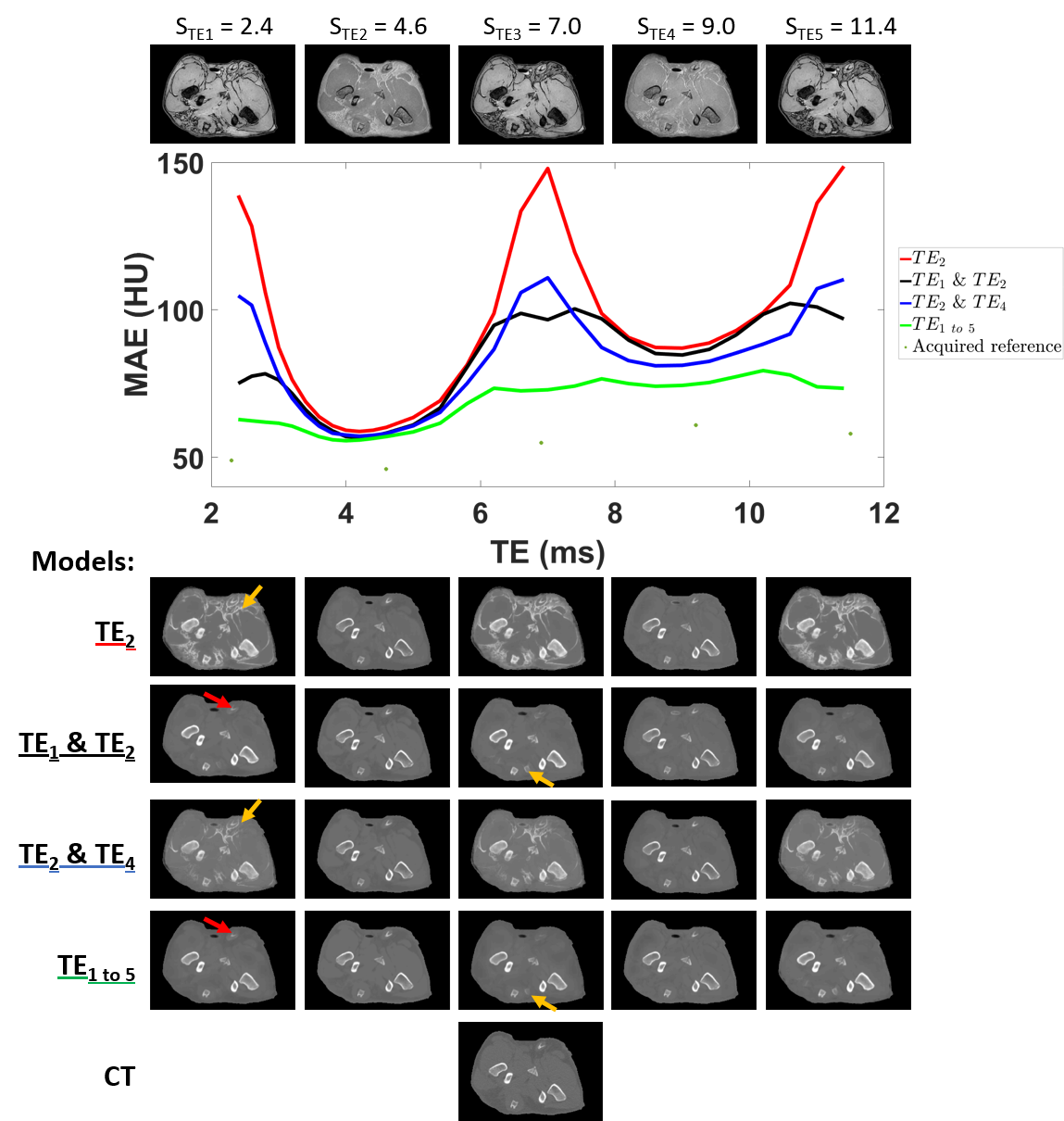
Figure 4 shows the evolution of model performance on images simulated at multiple TEs. The performance of a model trained on a single TE (Seq1-TE2) was rapidly compromised when applied on different TEs. However, TE-augmentation improved prediction performance at different TEs with the model trained on all echoes providing the best generalization.
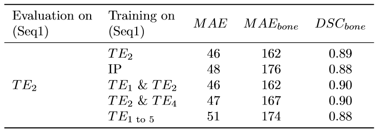
However, when evaluating on Seq1-TE2, TE-augmentation came with a slight performance penalty compared to models trained specifically on Seq1-TE2 (Figure 5).
Discussion and conclusion
In this study, we showed that models tended to perform adequately only on the very specific echo times of the training images. Performing TE-augmentation during training improved the generalizability of such models to different echo times but compromised the performance for any single TE.
Despite being focused on echo times, this study established the adverse effect of transferring a model from one image with specific acquisition parameters to a slightly different image. In a clinical setting, even larger differences in image acquisition can be expected, including varying field strengths, repetition times or vendors. Hence, this study calls for better generalization of deep learning models to acquisition parameters.
Acknowledgements
The authors would like to acknowledge the support of NVIDIA Corporation with the donation of GPU for this research. This work is part of the research program Applied and Engineering Sciences (TTW) with project number 15479 which is (partly) financed by the Netherlands Organization for Scientific Research (NWO).References
1. Edmund JM, Nyholm T. A review of substitute CT generation for MRI-only radiation therapy. Radiation Oncology. 2017;12(1):28. doi:10.1186/s13014-016-0747-y
2. Dixon WT. Simple proton spectroscopic imaging. Radiology. 1984;153(1):189–94. doi:10.1148/radiology.153.1.6089263
3. Eggers H, Brendel B, Duijndam A, Herigault G. Dual-echo Dixon imaging with flexible choice of echo times. Magnetic Resonance in Medicine. 2011;65(1):96–107. doi:10.1002/mrm.22578
4. Klein S, Staring M, Murphy K, Viergever MA, Pluim JPW. Elastix: A toolbox for intensity-based medical image registration. IEEE Transactions on Medical Imaging. 2010;29(1):196–205. doi:10.1109/TMI.2009.2035616
5. Hamilton G, Yokoo T, Bydder M, Cruite I, Schroeder ME, Sirlin CB, Middleton MS. In vivo characterization of the liver fat 1H MR spectrum. NMR in Biomedicine. 2011;24(7):784–790. doi:10.1002/nbm.1622
Figures