Synopsis

Rician noise represents the major source of bias in parametric fitting techniques, such as the estimation of the T₂* relaxation time. This bias is particularly strong when the signal-to-noise ratio is low or T₂* values are short, such as in clinical cases of severe brain or liver iron overload. In this work, we trained a deep convolutional neural network to recognize Rician noise and compute unbiased relaxation parameters from multi-echo gradient echo data.

Introduction

Noise on MR magnitude images follows a Rician distribution, which means that the noise level and its mean depend on the signal intensity.¹ Several studies have demonstrated that Rician noise represents the major source of bias in parametric fitting techniques, such as the estimation of the T₂* relaxation time.^8-12 This bias is particularly strong when the signal-to-noise ratio is low or T₂* values are short, such as in clinical cases of severe brain or liver iron overload.

Several methods have been proposed to address Rician noise bias, such as the Power Method,^2,3 echo train truncation,^4,5 and the incorporation of an additional offset fitting parameter.^6,7 However, these approaches suffer from their own intrinsic biases because they do not model the Rician noise distribution properly.^8-12

In this work, we trained an artificial neural network to recognize Rician noise and compute unbiased relaxation parameters from multi-echo gradient echo data.

Methods

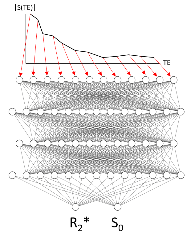
Network Architecture: We built an artificial neural network (ANN) with three fully connected hidden layers and rectifying linear unit (ReLU) activation functions in Keras 2.2.0 (12 input nodes, 13*, 12*, and 13* hidden nodes, and two output nodes; * indicates an extra bias node per layer). The model architecture is illustrated in Figure 1.

Training Data Simulation: We used simulated signal decay curves to train the ANN. We simulated mono-exponential decay curves with R₂* (=1/T₂*) between 0 and 400/s (T₂*>2.5ms), maximum signal intensity between 0 and 2 [a.u.], and signal-to-noise ratios (SNRs) between 2 and 40. All parameters were chosen randomly (uniformly distributed) from within the stated intervals. The Rician noise was simulated by adding Gaussian noise to the real and imaginary components of the signal. We mimicked 12 gradient echoes with TE₁=4.76ms and ΔTE=3.96ms.

Network training: We trained the network (GPU; NVIDIA GeForce GTX 750 Ti) with the Adam Optimizer (Tensorflow 1.8) using mean squared error loss and data shuffling with 10 million decay curves. We used 100,000 decay curves for the validation.

Conventional methods: For comparison purposes, we applied the following conventional fitting techniques (all logarithmic calculus) to the validation data: direct fitting; fitting of the squared signal after noise correction (“Power Method”); and echo truncation at SNR values below 2, 4, 8, 16, and 32.

MRI: The proposed method was evaluated in vivo using clinical multi-echo gradient echo data acquired at 3 Tesla (same echo times as used for training data generation). Relaxation rate constants were calculated on a voxel-by-voxel basis.

Results

Training and evaluation losses decreased monotonically during the first 4000 epochs and converged to below 1% relative difference. We stopped the training after 6500 epochs.

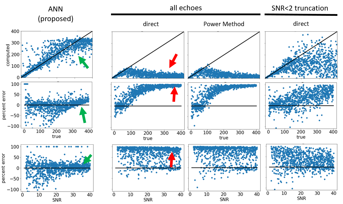
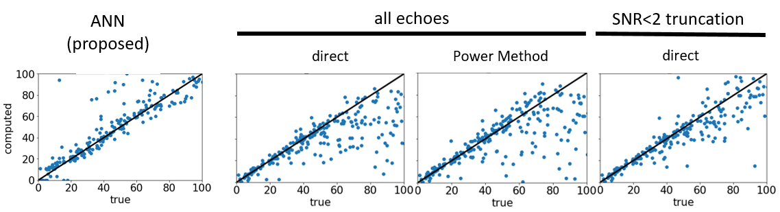
Figure 2 compares the performance of the proposed method with the conventional methods over the full range of R₂* and SNR values in the validation data. The conventional methods substantially underestimated R₂* when true values fell below 100/s (T₂*<10ms) independent of the SNR (red arrows). The proposed method estimated the true R₂* values linearly up to 300/s (T₂*>2.8ms). Figure 3 enlarges a randomly chosen subset of samples with R₂* values that are typically observed in brain MRI at 3T, which demonstrates underestimation in low SNR regimes even for these moderate relaxation rates.

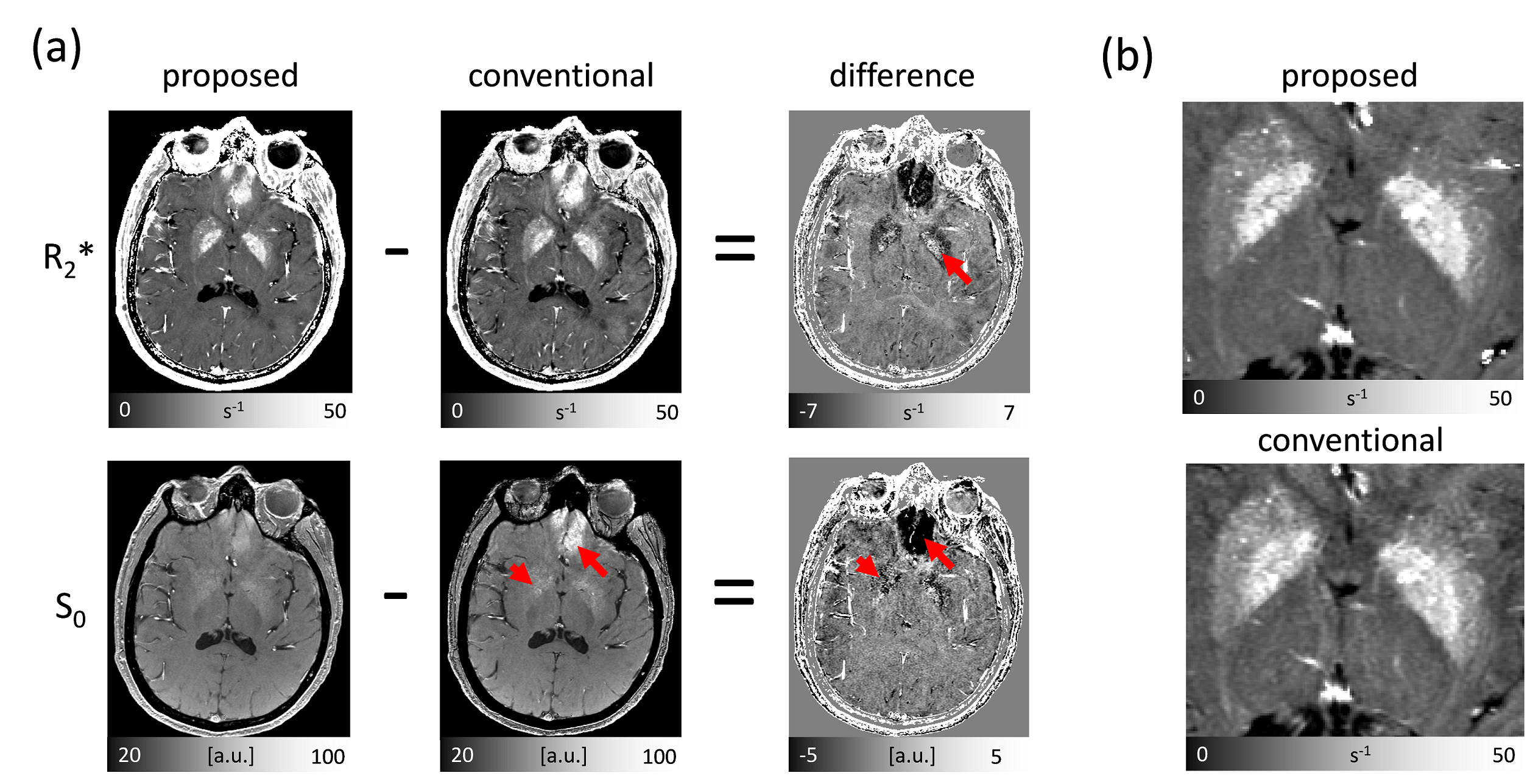
Figure 4 demonstrates the applicability of the proposed method in the clinical setting and illustrates decreased bias compared to conventional techniques in the iron-laden subcortical gray matter. Furthermore, the comparison revealed that the proposed technique yielded parameter maps with a reduced noise level, probably due to a more appropriate modeling of the underlying noise distribution.

The computation time for the 3D in vivo MRI scan was below 100 seconds on a workstation without GPU (CPU only).

Discussion

The non-linearity of artificial neural networks with non-linear activations allows modeling the Rician noise distribution correctly in the mono-exponential parameter-fitting problem and, hence, substantially extends the range of R₂* values that can be obtained reliably with a chosen multi-echo train. The non-linear relationship between quantified and actual R₂* values were successfully resolved.

In this work, we used only simulated signal curves for the network training, providing full control over the training process and potential training bias. Depending on the particular sequence parameters, the proposed method will help obtain more reliable estimations of the iron load in the brain and promises to yield more robust clinical estimations of liver iron content in iron overload conditions.

Conclusion

Acknowledgements

References

1. Gudbjartsson H and Patz S. Magn Reson Med, 34(6):910–914, 1995.

2. Miller AJ and Joseph PM. Magn Reson Imaging, 11(7):1051–6, 1993.

3. Raya JG et al. Magn Reson Med, 63(1):181–93, 2010.

4. Yin X et al. NMR Biomed, 23(10):1127–36, 2010.

5. He T et al. Magn Reson Med, 60(2):350–6, 2008.

6. Du G et al. PLoS One, 7(4):e35397, 2012.

7. Ghugre NR et al. J Magn Reson Imaging, 23(1):9–16, 2006.

8. Beaumont M et al. J Magn Reson Imag, 30(2):313–20, 2009.

9. Feng Y et al. Magn Reson Med, 2013.

10. Marro K et al. Magn Reson Imaging, 29(4):497–506, 2011.

11. Raya JG et al. Magn Reson Med, 63(1):181–93, 2010.

12. Otto R et al. Pediatr Radiol, 41(10):1259–65, 2011.