4851
Deep Neural Networks for Motion Estimation in k-space: Applications and Design1Pattern Recognition Lab, Friedrich-Alexander University Erlangen-Nürnberg, Erlangen, Germany, 2Siemens Healthineers AG, Erlangen, Germany, 3Martinos Center for Biomedical Imaging, Charlestown, MA, United States
Synopsis
While image-based motion estimation with Deep Learning has the advantage of an easier comprehension by a human observer, there are benefits to address the issue in k-space, as the distortion only affects echo trains locally; furthermore, Neural Networks can be designed to rely on the intrinsic k-space structure instead of image features. To our knowledge, these advantages have not been exploited so far. We show that fundamental Deep Neural Network techniques can be used for motion estimation in k-space, by examining different networks and hyperparameters on a simplified problem. We find suitable architectures for extracting 2D transformation parameters from under-sampled k-spaces for slice registration. This leads to a minimum residual of around 1.2 px/deg.
Introduction
Deep Learning (DL) is widely investigated in the context of MRI, for example in segmentation1 or reconstruction2,3,4. In image space, reconstructions are refined2 using DL; in k-space current DL is limited to reconstruction3,4. For motion detection in k-space Random Forests are used5. Motion detection and estimation in k-space using DL seem counterintuitive at first, as convolutional layers mostly learn edge detection and derived higher-order features; this aspect cannot be easily extrapolated to k-space. Furthermore, the centrally aligned value distribution is not well suited for DL.
However, k-space holds some unique properties which, for example, encode relevant information for motion estimation. In fact, direct processing of k-space can exploit two advantages, which are 1) specific to the MRI acquisition and 2) purely algorithmic:
- In acquisition domain, the order of filling the k-space encodes temporal information. Furthermore, temporal effects, such as motion, affecting each echo train differently are local in contrast to image domain where these effects result in global changes.
- Due to absence of image features, Neural Networks (NNs) must rely on k-space properties. In motion, these properties are phase shifts and rotations of the Fourier coefficients.
Thus, we expect DL in k-space to be better suited for motion problems, by learning the mathematical and temporal connection of the Fourier domain and its acquisition. To test the theoretical approach along with analyzing suitable NNs for k-space problems, a simplified motion problem is constructed. We investigate common NNs for solving this task, by varying their hyperparameters, and draw conclusions about the general initial design of NNs for k-space motion extraction.
Methods
The underlying task is to solve a simple registration problem due to motion between two identical sequences by extracting the inplane transformation parameters.
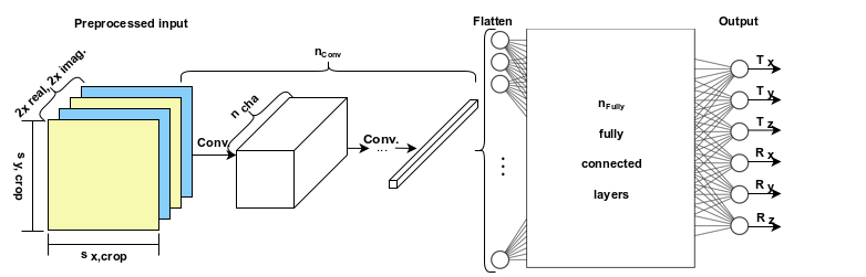
For training and validation data creation, a simulation was performed by applying random translations with phase ramps Δx, Δy and rotations φ, all within a range of [-12..12] px/deg to acquired k-spaces with a matrix size of 448 and FOV of 220 mm. The data from phantoms and volunteers were acquired with a 3T Siemens MAGNETOM Prisma (Siemens Healthcare, Erlangen, Germany). To simulate under-sampling, every second row was removed. The complex data was fed into the network as 4 individual channels using a central cropped patch with size sx,crop, sy,crop.
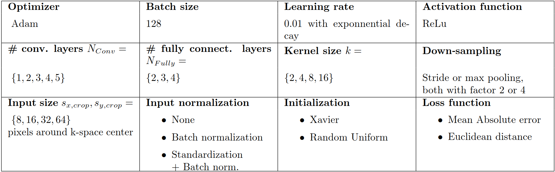
The baseline architecture is depicted and explained in Figure 1. The detected motion parameters were compared in the loss function to the normalized ground truth. A random fraction of all combinations of the hyperparameters, including sx,crop, sy,crop, described in Table 1, were trained after excluding some in prior tests. Subsequently, the networks were analyzed for overall convergence, speed of convergence, and minimum residuals during limited training time. Afterwards, one of the most promising networks was picked and trained until no significant improvements were obtained by incorporating findings made during the hyperparameter search.
Results
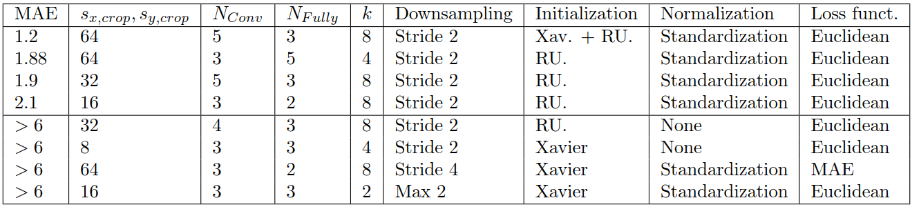
A selected subset of various training results can be seen in Table 2. It indicates, that an input size sx,crop, sy,crop ≥ 2*k and kernel size k between 4 and 8 is crucial. A down-sampling of 2, independent of strided convolutions or max pooling shows better results than higher values. Standardization for each sample and batch normalization were beneficial as preprocessing. In our experiments, using the popular Xavier initialization resulted in slow or no convergence. This was improved by using random uniform initialization between ± 0.075 for the fully connected part, as Xavier results in too small initial weights. Every architecture w.r.t. NConv and NFully, with NConv, NFully ≥ 2 for enough capacity, converged to a solution, provided that all above described conditions were met.
The mean absolute error (MAE) as loss function did not result in convergence in prior tests; therefore, the Euclidean distance (ED) was chosen. This has the additional advantage of also penalizing large errors more, as these large errors might worsen the final image after correction.
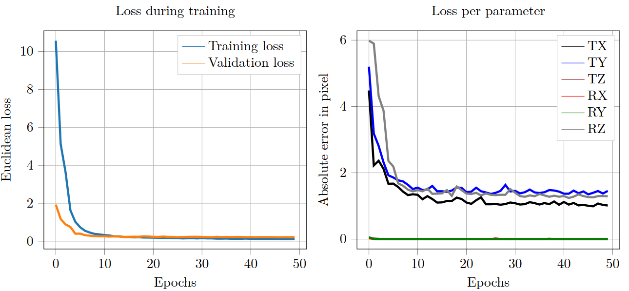
The first row of Table 2 shows the network, which was optimized within the generic simple NN architecture by using the above described initialization scheme and increased number of epochs. The training process, depicted in Figure 2, resulted in a MAE of 1.2 px/deg per parameter. This shows that NNs can approximate motion, applied as phase shifts and rotations, and a deeper investigation seems promising.
Conclusion and Outlook
The presented method of using a combination of simple operators to tackle tasks in k-space domain shows encouraging results for k-space-based motion estimation, even if under-sampling was applied. However, using k-space needs additional attention on the initialization, the kernel size, and the preprocessing.
Further steps include the fine-tuning of networks to improve the performance and to generalize the networks to detect advanced motion patterns.
Acknowledgements
No acknowledgement found.References
1Işına A., Direkoğlub C., Şahc M. Review of MRI-based brain tumor image segmentation using deep learning methods. 12th International Conference on Application of Fuzzy Systems and Soft Computing, ICAFS 2016; 2016 August 29-30, Vienna, Austria
2Seitzer M., Yang G., Schlemper J., Oktay O., Würfl T, Christlein V., Wong, T., Mohiaddin R., Firmin D., Keegan J., Rueckert D., Maier A. Adversarial and Perceptual Refinement for Compressed Sensing MRI Reconstruction. Medical Image Computing and Computer Assisted Intervention – MICCAI 2018 (MICCAI 2018), Granada, Spain; 2018 Sept 16, pp. 232-240, 2018, ISBN 978-3-030-00928-1
3Hammernik, K., Klatzer, T., Kobler, E., Recht, M. P., Sodickson, D. K., Pock, T., & Knoll, F. (2018). Learning a variational network for reconstruction of accelerated MRI data. Magnetic resonance in medicine, 79(6), 3055-3071.
4Zhu B., Liu J., Cauley S., Rosen B., Rosen M. Image reconstruction by domain-transform manifold learning. Nature. 2018 Mar 21; 555(7697): pp. 487-492
5Lorch B., Vaillant G., Baumgartner C., Bai W., Rueckert D., Maier A. Automated Detection of Motion Artefacts in MR Imaging Using Decision Forests. Journal of Medical Engineering, vol. 2017, no. 4501647, pp. 1-9, 2017
Figures