4845
3D MRI Denoising with Wasserstein Generative Adversarial Network1College of Computer Science, Sichuan University, Chengdu, China, 2Department of Computer Science, Chengdu University of Information Technology, Chengdu, China, 3Lab of Image Science and Technology, Southeast University, Nanjing, China, 4Department of Radiology, West China Hospital of Sichuan University, Chengdu, China
Synopsis
MR image is easily affected by noise during the high-speed and high-resolution acquisition procedure. To effectively remove the noise and fully explore the potential of latest technique -- deep learning, in this abstract, we propose a novel MRI denoising method based on generative adversarial network. Specifically, to explore the structure similarity among neighboring slices, 3-D configuration are utilized as the basic processing unit. Residual autoencoder, combined with deconvolution operations are introduced into the generator network. The experimental results show that the proposed method achieves superior performance relative to several state-of-art methods in both noise suppression and structure preservation.
Introductions
Magnetic resonance imaging (MRI) plays an important role in current clinical diagnosis. However, when high-speed and high-resolution is needed, the reconstructed images will be heavily contaminated by noise. The existing MRI denoising methods are roughly divided into three categories based on spatial domain, frequency domain or statistical properties respectively1. These methods suffer from different shortcomings, including computational burden, structure loss, parameter selection, etc.
Large-scale applications of deep learning in computer vision and image processing suggest new thinking and huge potential for the medical imaging field. Several pioneering methods on deep learning for medical image restoration have been developed2, 3, but the researches for MRI denoising are quite limited. In this abstract, we propose a 3D MRI denoising method based on Wasserstein generative adversarial network.
Methods
The aim of MRI denoising is to recover a high-quality MR image from the corresponding noisy MR image. Let $$$x\in\mathbb{R}^{m \times n}$$$ and $$$y\in\mathbb{R}^{m \times n}$$$ denote the noisy MR image and the corresponding noise-free MR image respectively. MR denoising can be simplified to seek an optimal mapping function $$$f$$$:
$$f=\arg\min\limits_{f}||f(x)-y||_2^2$$
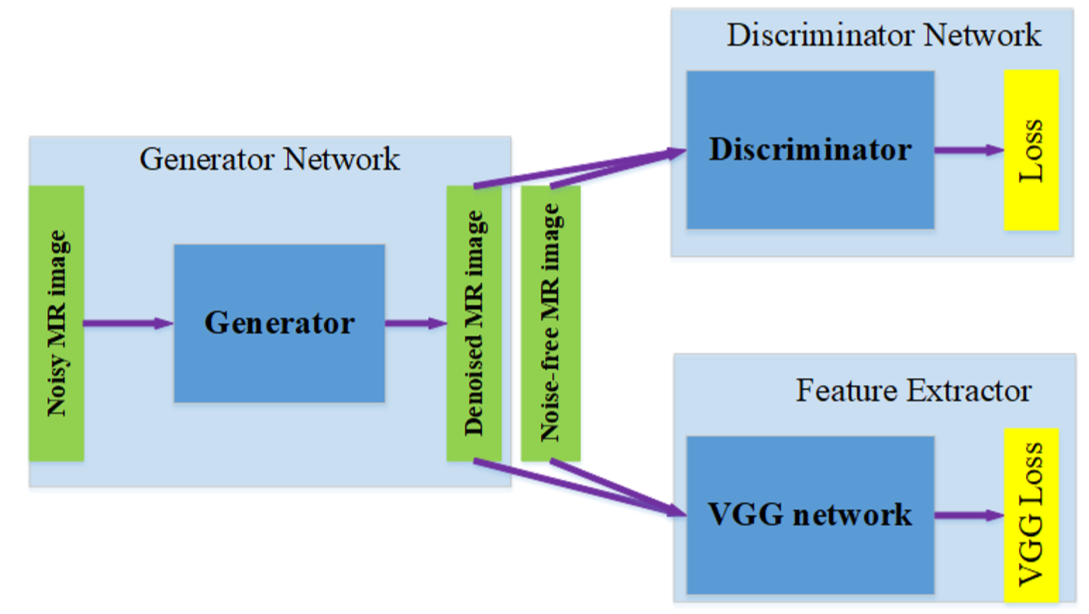
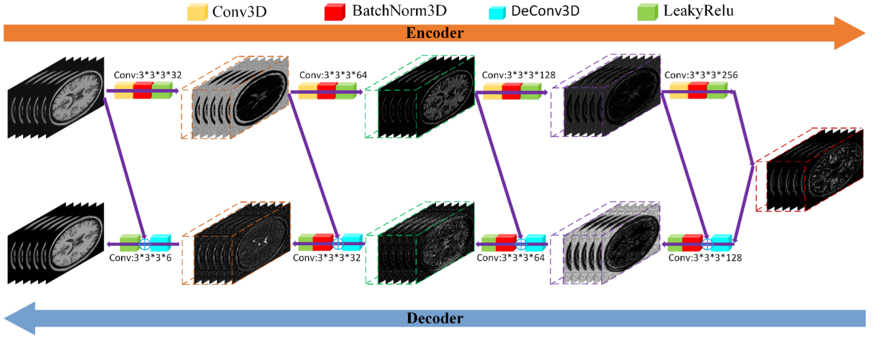
DL-based methods are independent of the statistical characteristic of noise in image domain and efficient in image restoration. Following this direction, we propose a novel 3D MRI denoising method based on Wasserstein generative adversarial network (WGAN) which called RED-WGAN and the overall architecture of RED-WGAN is illustrated in Fig. 1. RED-WGAN takes WGAN as fundamental framework. The specific structure of generator network G is demonstrated in Fig. 2. The residual autoencoder, combined with deconvolution operations are introduced into G to accelerate the training procedure and preserve more details. G is an encoder-decoder structure, which is made up of 8 layers, including 4 convolutional and 4 deconvolutional layers, and the convolution and deconvolution layers are symmetrically arranged. Short connections link the corresponding convolution-deconvolutional layer-pairs. Furthermore, to alleviate the shortcoming of traditional mean-squared error (MSE) loss function for over-smoothing, the perceptual similarity, which is implemented by calculating the distances in the feature space extracted by a pre-trained network, is incorporated with MSE and adversarial loss to form the hybrid loss function of G, which is formulated as:
$$L_{RED-WGAN}(G)=\lambda_1\frac{1}{W_1H_1D_1}||G(x)-y||^2 + \lambda_2\frac{1}{W_2H_2D_2}||VGG(G(x))-VGG(y)||^2_F-\lambda_3\mathbb{E}[D(G(x))]$$
where $$$λ_1,λ_2,λ_3$$$ are belance factors, $$$W_1,H_1,D_1$$$ and $$$W_2, H_2, D_2$$$ stand for the dimensions of the image and the feature map respectively, G is the generator, D is the discriminator, and VGG is the feature extractor from a pre-trained VGG-19 network. The proposed loss function is composed of three parts: the first item is the MSE loss, the second is the perceptual loss and the last one is the adversarial loss.
D is a simple end-to-end network which contains three convolutional layers and a full-connected layer and its loss function is defined as:
$$L_{RED-WGAN}(D)=-\mathbb{E}[D(y)] + \mathbb{E}[D(G(x))]+\lambda\mathbb{E}[(\|\nabla_{\hat{x}}D(\hat{x}) \|_2-1)^2]$$
where $$$\hat{x}=\epsilon y+(1-\epsilon)G(x)$$$, $$$\lambda$$$ is the gradient penalty coefficient, $$$\epsilon$$$ is a random variable sampled from $$$U[0,1]$$$.
Results
In the experiments, the parameters $$$λ,λ_1,λ_2,λ_3$$$ were experimentally set to 10, 1, 0.1 and 1e-3 and Adam was utilized to optimize the loss function. The dataset comes from the well-known IXI dataset4 and 50000 cubes with size of 32×32×6 are extracted by a fixed sliding step.
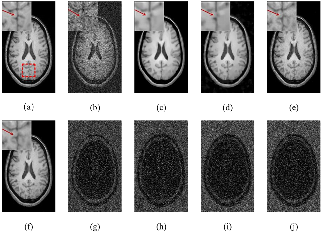
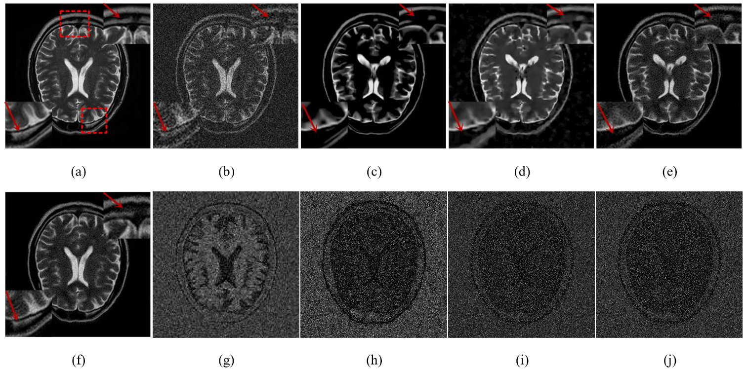
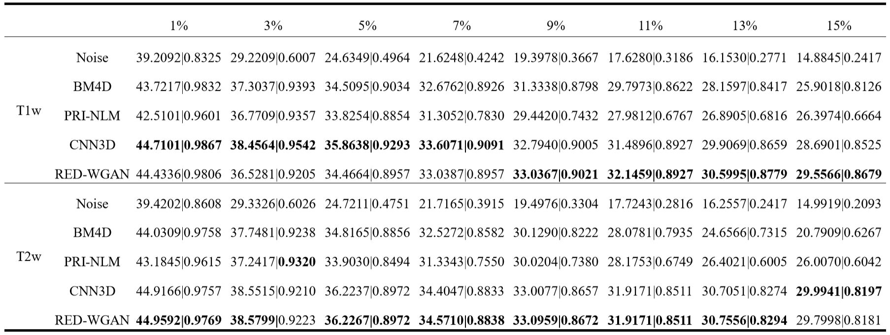
To validate the performance of the proposed RED-WGAN, three methods, including CNN3D (only generator part of RED-WGAN and MSE loss), BM4D5 and PRI-NLM6 were compared and two quantitative metrics, PSNR and SSIM, were employed. The average quantitative results of all methods on T1w and T2w images with different noise levels from 1% to 15% with a step of 2% are illustrated in Tables I. Figs. 3 and 4 provide a visual evaluation of different methods on T1w and T2w brain images corrupted with 15% Rician noise, respectively.
Discussion and Conclusion
In Table I, it can be observed that the performances of DL-based methods are superior to current denoising algorithms on both PSNR and SSIM. In Figs. 3 and 4, BM4D and PRI-NLM suffer from obvious over-smoothing effect and distort some important details, both RED-WGAN and CNN3D avoid over-smoothing effect efficiently and preserve more structural details. It is also worth noting that although the scores of CNN3D are close to that of RED-WGAN, RED-WGAN obtained better visual effects and recovered more details, which is coherent to the previous observations3, 7.
In conclusion, the results obtained in the paper are encouraging and efficiently demonstrate the potentials of deep learning based methods for MRI denoising. In the future, instead of training on a specific noise level, we will try to extend our method to a more general form for different noise levels.
Acknowledgements
This work was supported in part by the National Natural Science Foundation of China under grants 61671312 and 61302028, the National Key R&D Program of China under grants 2017YFB0802300, the Science and Technology Project of Sichuan Province of China under grants 2018HH0070.References
1. J. Mohan, V. Krishnaveni, and Y. Guo, "A survey on the magnetic resonance image denoising methods," Biomedical Signal Processing & Control, vol. 9, no. 1, pp. 56-69, 2014.
2. H. Chen et al., "Low-dose CT with a residual encoder-decoder convolutional neural network (RED-CNN)," IEEE Transactions on Medical Imaging, vol. PP, no. 99, pp. 1-1, 2017.
3. Q. Yang et al., "Low-dose CT image denoising using a generative adversarial network with Wasserstein distance and perceptual loss," IEEE Transactions on Medical Imaging, vol. 37, no. 6, pp. 1348-1357, 2017.
4. http://brain-development.org/ixi-dataset/
5. M. Maggioni, V. Katkovnik, K. Egiazarian, and A. Foi, "Nonlocal transform-domain filter for volumetric data denoising and reconstruction," IEEE Transactions on Image Processing, vol. 22, no. 1, pp. 119-133, 2012.
6. J. V. Manjón, P. Coupé, A. Buades, C. D. Louis, and M. Robles, "New methods for MRI denoising based on sparseness and self-similarity," Medical Image Analysis, vol. 16, no. 1, pp. 18-27, 2012.
7. C. Ledig et al., "Photo-Realistic Single Image Super-Resolution Using a Generative Adversarial Network," in CVPR, 2017, vol. 2, no. 3, p. 4.
Figures