Synopsis

Conventional denoising and noise level estimation typically require data redundancy from multiple measurements or prior assumptions, such as smooth image prior or similarity between image patches. Here, we propose a single image denoising algorithm with noise map estimation by identifying the noise-only principle components based on universal properties of random covariance matrices, with the data redundancy created by segmenting data in the Fourier or wavelet domains. The proposed method is applicable to medical and other imaging modalities with spatially-varying noise, and is particularly beneficial to quantitative MRI acquisitions with a limited number of scans.

Purpose

Denoising is essential for reliable image processing (e.g.,co-registration, super-resolution,etc.)[1]. In particular, estimating the image noise level is necessary for image reconstruction in compressed sensing[2]. To date, denoising and noise level estimation requires either data redundancy from multiple measurements (empirically>30)[3,4] or prior assumptions, such as smooth image prior[1] or similarity between image patches[5,6]. However, neither of these two conditions can be satisfied for some applications.

Here, to achieve single image denosing and noise level/map estimation without prior assumptions, we propose an algorithm to identify the noise-only principal components using universal properties of the random covariance matrix[3,4], for which the required data redundancy is created by stacking re-ordered Fourier transformed (k-space) or wavelet-transformed patches from the single image. This empirical redundancy serves as a ground for the denoising at a single-image level, enabling the separation between image features and the noise. This method is universally applicable to images with spatially-varying noise, not just for medical (e.g.,MRI), but also for other imaging modalities (e.g.,electron microscopy).

Methods

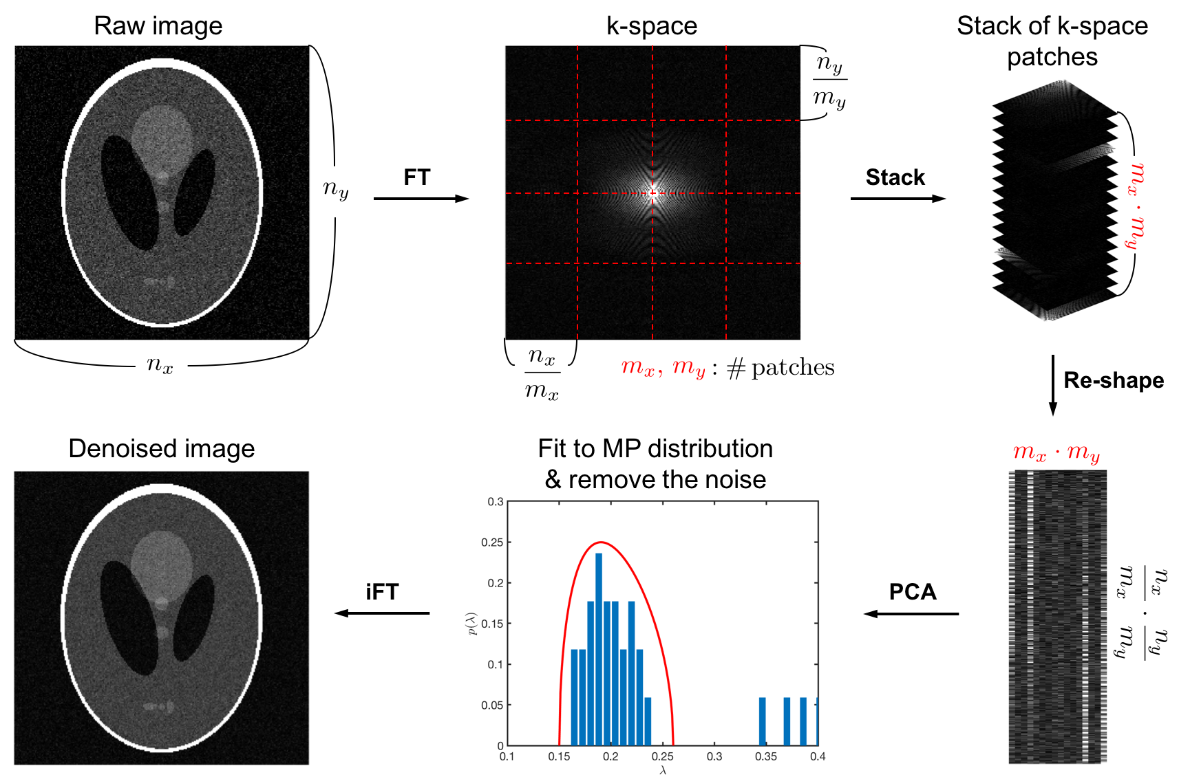
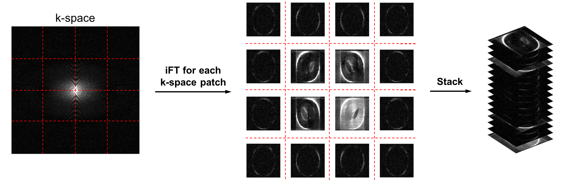
$$$\rm\bf{Denoising\,algorithm,\,Figs.1\text{-}2}$$$

Consider a $$$d$$$-dimensional image ($$$n$$$ voxels in total) corrupted by noise (e.g., Gaussian, Poisson, Rician). First, we perform the Fourier transform (FT) of the raw image, and segment the k-space data into $$$m_1$$$,$$$m_2$$$, ...,$$$m_d$$$ equal parts along each dimension respectively. Then we stack the segmented k-space data to create the data redundancy (Fig.2) by a factor of $$$m=\prod_{i=1}^dm_i$$$, and re-shape the stacked data into an $$$\frac{n}{m}$$$×$$$m$$$ redundant matrix $$$\bf{X}$$$ with P (presumably $$$\ll$$$min$$$(\frac{n}{m},m)$$$) linearly independent components. After applying the principal component analysis (PCA) to the matrix $$$\bf{X}$$$, the smallest min$$$(\frac{n}{m},m)$$$-P nonzero eigenvalues are purely contributed by the noise and obey the Marchenko-Pastur (MP) distribution[7]. Finally, we remove the noise components identified by MP distribution in PCA domain, unstack the data, and perform inverse-FT (iFT) to obtain the denoised image. As opposed to non-local means methods[5,6], we do not need ad hoc similarity criterion; rather, MP-PCA sets such a criterion automatically and objectively.

In actual implementations, FT can be replaced by other orthonormal transformations, such as the wavelet transform (WT). The FT-approach can estimate only the general noise level for the whole image. In contrast, the WT-approach, combined with a sliding window (kernel), can estimate a spatially dependent noise map with lower resolution.

$$$\rm\bf{Residual\,analysis}$$$

To test the performance of our denoising method, we analyzed the normalized residual $$$r$$$ of the raw image $$$I$$$ and the denoised image $$$I^\prime$$$[3-4], defined by

$$r\equiv\frac{I^\prime-I}{\sigma}\quad\quad(1)$$

with $$$\sigma$$$ the estimated noise level/map. The normalized residual should be normal distributed with a zero mean and a variance ≤1 when the denoising algorithm removes only the noise, without corrupting the signal.

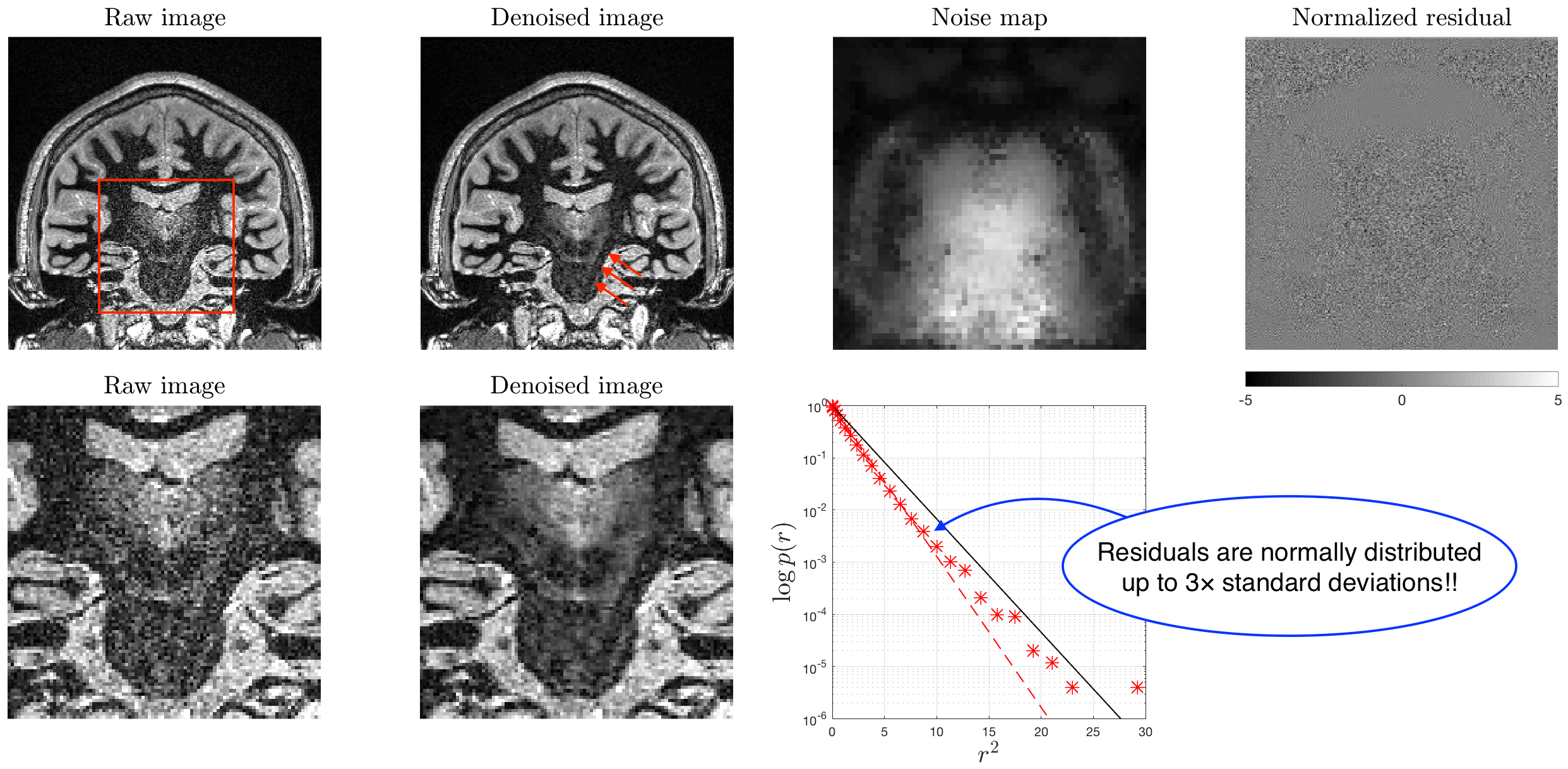
$$$\rm\bf{Data\,1:\,T_1\text{-}weighted\,3D\,FGATIR\,MRI\,(single\,image\,in\,3d),\,Fig.3}$$$

We scanned a 20s-year-old female on a 3T-Siemens-Prisma using the T$$$_1$$$-weighted 3D-FGATIR sequence (Fast-Gray-Matter-Acquisition-T$$$_1$$$-Inversion-Recovery, resolution=(0.8mm)$$$^3$$$, FOV=179×230mm$$$^2$$$, TE/TR=4.39/3000ms, TI=409ms, acquisition time=11min), and denoised the brain image using level-2 WT-approach in 3d with a 5×5×5-kernel.

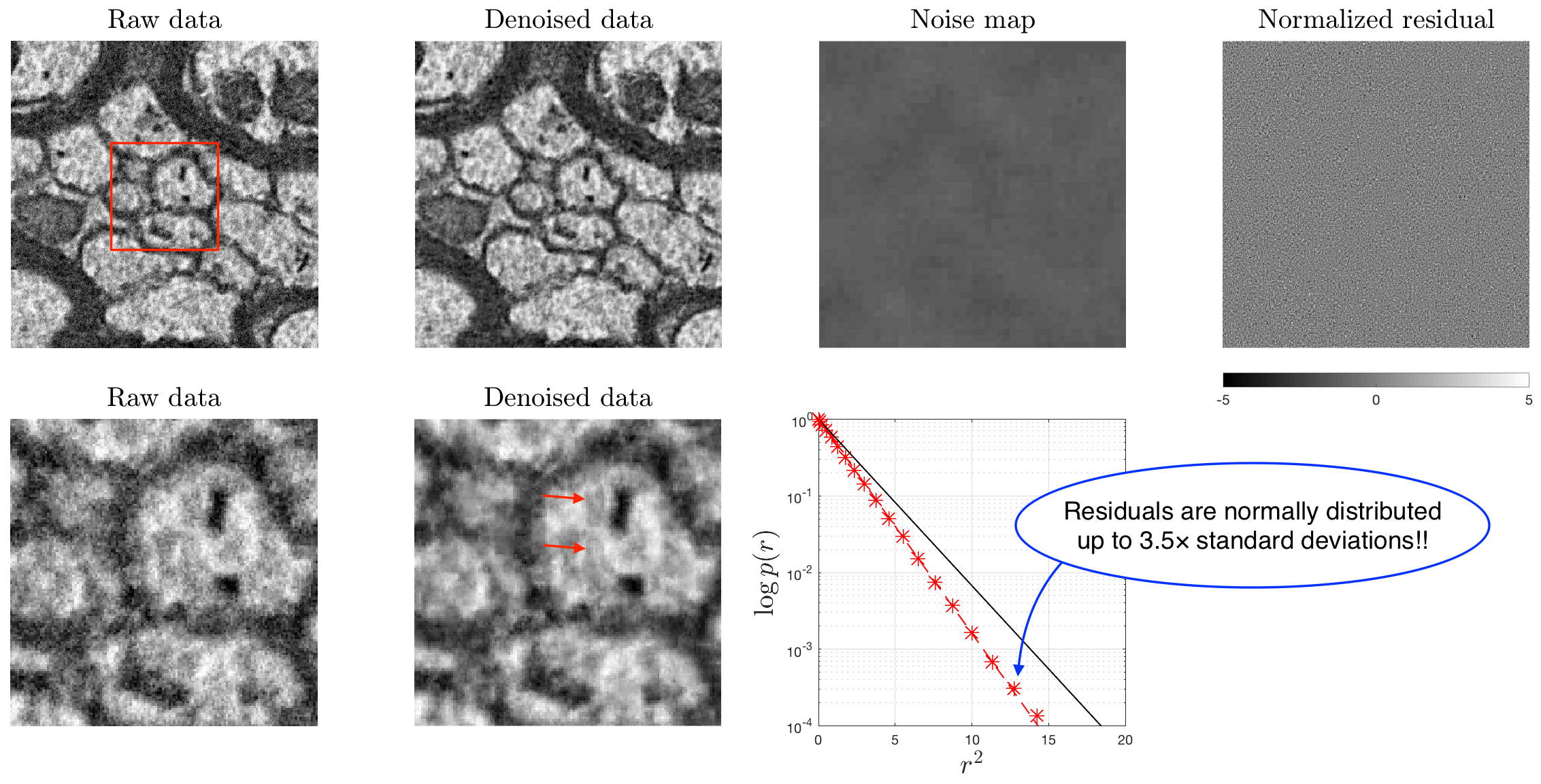
$$$\rm\bf{Data\,2:\,Scanning\,electron\,microscopy\,(SEM)\,(single\,image\,in\,2d),\,Fig.4}$$$

The brain tissue from a female 8-week-old C57BL/6 mouse’s genu of corpus callosum was processed and analyzed with an SEM (Zeiss Gemini-300) in a 6×6nm$$$^2$$$ pixel size[8]. We demonstrated our denoising method on a 400×400 data matrix, using level-3 WT-approach in 2d with a 7×7-kernel.

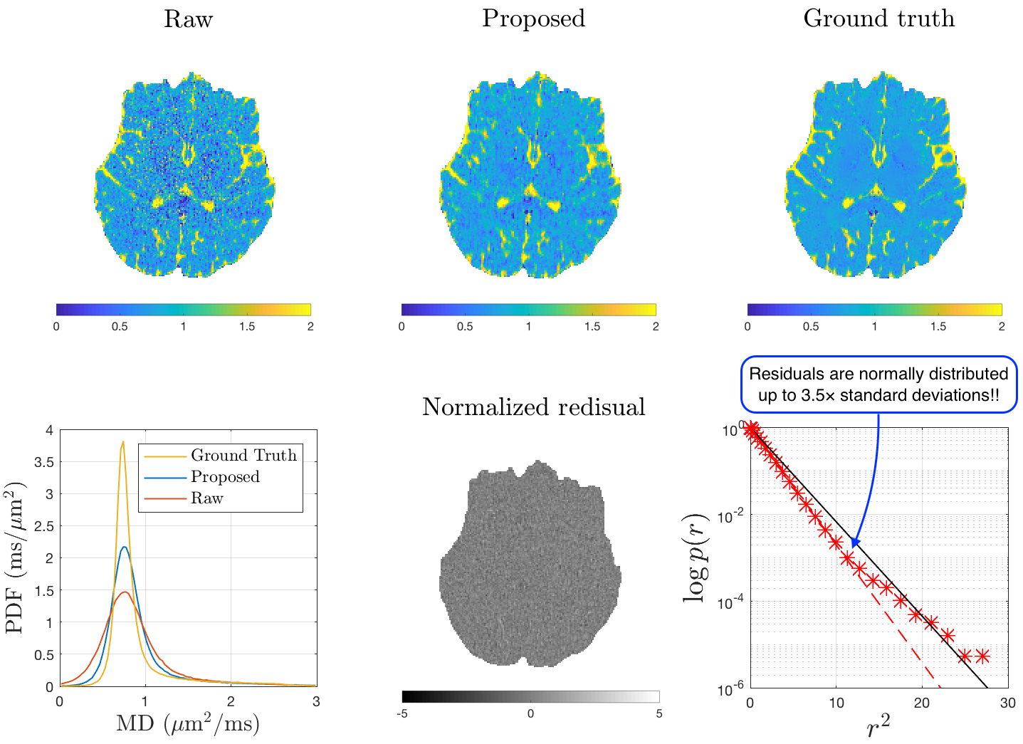
$$$\rm\bf{Data\,3:\,Diffusion\,MRI\,(4\,images\,in\,3d),\,Fig.5}$$$

We scanned a 24-year-old female on a 3T-Siemens-Prisma and acquired 1b=0 brain image and 3DWIs with b-value=1000s/mm$$$^2$$$ (resolution=(1mm)$$$^3$$$, FOV=182×184mm$$$^2$$$, TE/TR=68/5200ms, PF=5/8), and denoised the 4 images using level-2 WT-approach in 3d with a 5×5×5-kernel. Further, we acquired 3b=0 images and 30DWIs using the same sequence, and denoised the 33 images using the ordinary MP-PCA (dwidenoise, mrtrix, 5×5×5-kernel)[3,4] as the ground truth. Total acquisition time is 10min. We compared the mean diffusivity (MD) map for raw data, denoised data with proposed method, and the ground truth.

Results

In Fig.3, compared with the raw image acquired by FGATIR, the denoised image shows better contrasts for tracts (dark), e.g., corticospinal tract passing through the pons. The noise map is homogenous over the central region. The normalized residual map shows no structure, and its histogram is close to and below the normal distribution (zero-mean, variance=1), indicating that our method removes most of the noise without corrupting the signal. The SEM image in Fig.4 shows similar results.

In Fig.5, compared with the MD map calculated from the raw data, the MD map calculated from the 4 denoised images using the proposed method is more homogenous and closer to the ground truth. The MD histogram shows that the proposed method increases the precision of the estimated parameter, indicated by the narrower MD distribution than the case of the raw data. The averaged normalized residual is homogenous with no anatomical structure, and its histogram is close to the normal distribution.

Discussion and Conclusions

Acknowledgements

References

1. Liu, Ce, et al. "Noise estimation from a single image." Computer Vision and Pattern Recognition, 2006 IEEE Computer Society Conference on. Vol. 1. IEEE, 2006.

2. Lustig, Michael, et al. "Compressed sensing MRI." IEEE signal processing magazine 25.2 (2008): 72-82.

3. Veraart, Jelle, Els Fieremans, and Dmitry S. Novikov. "Diffusion MRI noise mapping using random matrix theory." Magnetic resonance in medicine 76.5 (2016): 1582-1593.

4. Veraart, Jelle, et al. "Denoising of diffusion MRI using random matrix theory." NeuroImage 142 (2016): 394-406.

5. Buades, Antoni, Bartomeu Coll, and J-M. Morel. "A non-local algorithm for image denoising." Computer Vision and Pattern Recognition, 2005. CVPR 2005. IEEE Computer Society Conference on. Vol. 2. IEEE, 2005.

6. Manjón, José V., et al. "Adaptive non‐local means denoising of MR images with spatially varying noise levels." Journal of Magnetic Resonance Imaging 31.1 (2010): 192-203.

7. Marčenko, Vladimir A., and Leonid Andreevich Pastur. "Distribution of eigenvalues for some sets of random matrices." Mathematics of the USSR-Sbornik 1.4 (1967): 457.

8. Lee, Hong-Hsi, et al. "Electron microscopy 3-dimensional segmentation and quantification of axonal dispersion and diameter distribution in mouse brain corpus callosum." bioRxiv(2018): 357491.