4814
Classification of benign and malignant lymph nodes based on ex-vivo diffusion MRI data1Centre for Medical Image Computing, Department of Computer Science, University College London, London, United Kingdom, 2Champalimaud Research, Champalimaud Centre for the Unknown, Lisbon, Portugal
Synopsis
Developing non-invasive imaging technique for detection and characterisation of lymph nodes is an important topic in cancer research. Diffusion MRI (dMRI) appears to be a promising modality for this task. This work investigates the ability of dMRI to differentiate benign and malignant lymph nodes based on a rich, ex-vivo dataset, and aims to find which measurements provide the most differentiation power.
Introduction
Lymph Node (LN) staging is one of the main determinants of the management of rectal cancer patients, yet current imaging methods show limited accuracy for that purpose1. Diffusion MRI (dMRI) is becoming an increasingly important tool for non-invasive detection of malignant lymph nodes2-4 and potential characterization of their microstructure5.
This work investigates the ability of dMRI to differentiate benign and malignant lymph nodes based on a rich, ex-vivo dataset and aims to find which measurements provide the most differentiation power. We also compare the performance of different classification techniques: Logistic Regression (LR), Random Forest (RF), Deep Neural Network (DNN) and Convolutional Neural Network (CNN).
Methods
Institutional setting, approved by ethics committee: A total of 31 malignant nodes and 23 benign nodes (as defined by a dedicated pathologist) were included, originating from patients histopathologically staged as N+ after surgery with curative intent, without neoadjuvant therapy. The nodes were preserved in 4% formaldehyde and moved to a 1% PBS solution 24h before scanning.
Image acquisition: Nodal pairs were imaged with a 16.4T Bruker® scanner. Imaging parameters: slice thickness: 0.7mm, in-plane resolution: 0.14x0.14mm2, matrix size: 70x70, TR/TE: 2800/6.5 ms. Diffusion acquisition: stimulated echo acquisition mode (STEAM) experiments were performed with gradient duration δ=1ms and gradient separation Δ={5,10,20,40,70,100,150}ms for b-values of 500 and 1000 s/mm2 and Δ={10,20,30,50}ms for b-values of 1500 and 2000 s/mm2, resulting in 22 shells with 6 gradient directions for each shell.
Data analysis: A Diffusion Tensor (DT) was fitted voxelwise to each shell using the effective b matrix of the acquisition, and then mean diffusivity (MD) and fractional anisotropy (FA) were computed. This results in 44 features (22 shells x FA and MD) for each voxel. First, employing all features, we study the accuracy of LR, RF (TreeBagger function in Matlab with 100 trees and default parameters for classification) and a DNN (3 fully connected layers with 30, 5 and 1 node, respectively, implemented in Matlab). Then, to investigate the effect of including shape and texture we also analyse a CNN with the following architecture: C332-P-C310-D-P-C510-D-FC40-FC2-SL-CL, where CkN is a convolution layer with N filters of size k x k, P is a 2x2 max-pooling layer, D is a dropout layer, FCN is a fully-connected layer with N nodes, SL is a soft-max layer and CL is a classification layer; each convolution layer is followed by a batch normalization layer and a ReLU layer. The CNN is applied to 45 channels (44 diffusion features and the probability output of DNN). The dataset is split 80-20 for training and testing. Mean accuracy and its standard deviation is computed over 20 repetitions. We also study the importance of different features for classification based on RF, and the classification accuracy using four feature subsets.
Results
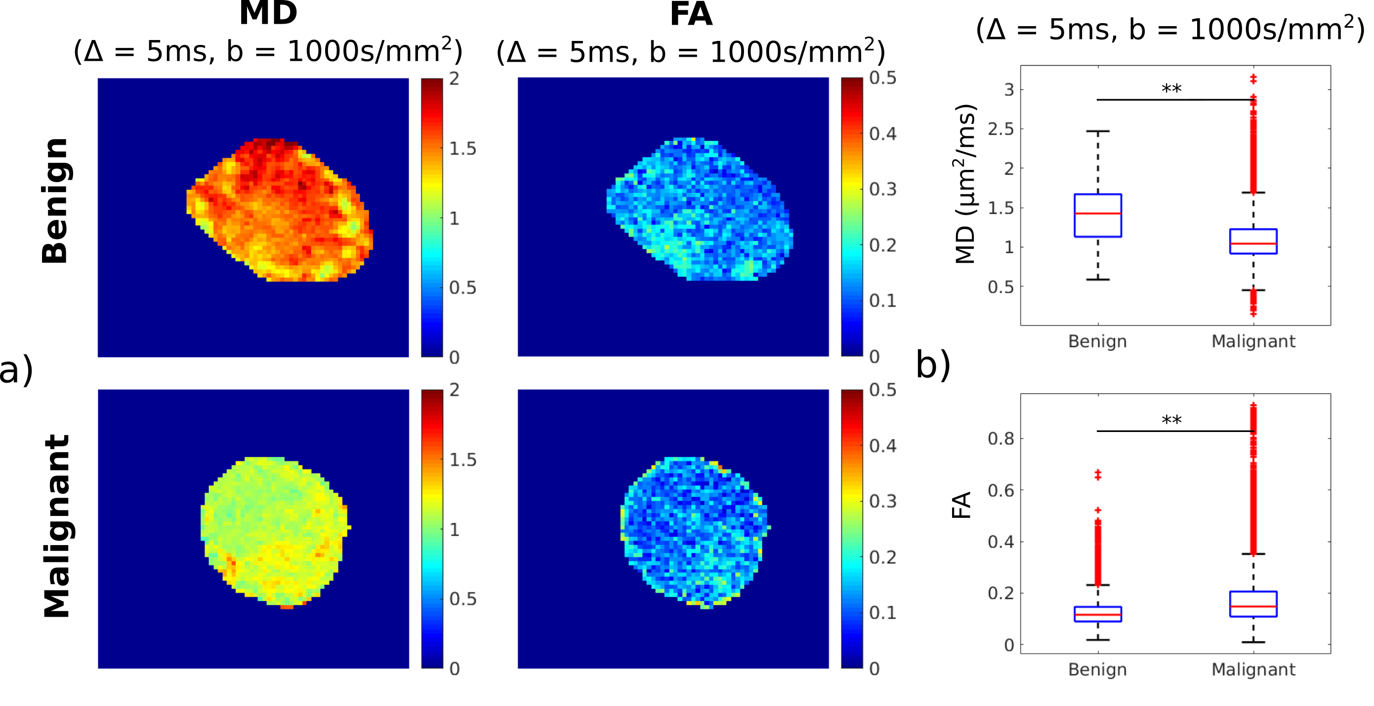
Figure 1 shows parameter maps of MD and FA for a benign and a malignant node (measured at Δ = 5ms and b = 1000 s/mm2) and boxplots of voxelwise MD and FA values in the two nodes, which are both statistically different (p<<0.01).
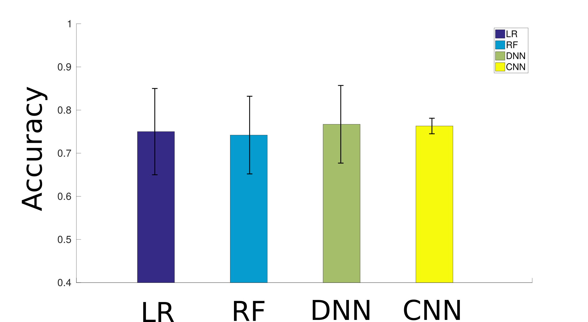
Figure 2 illustrates the classification accuracy and its uncertainty for LR (75.1±10.1%), RF (74.2±9.1%), DNN (76.6±9.2%) and CNN (76.3±1.3%) when employed with all 44 features. The uncertainty is around 10% for LR, RF and DNN, and much smaller (1.3%) for CNN.
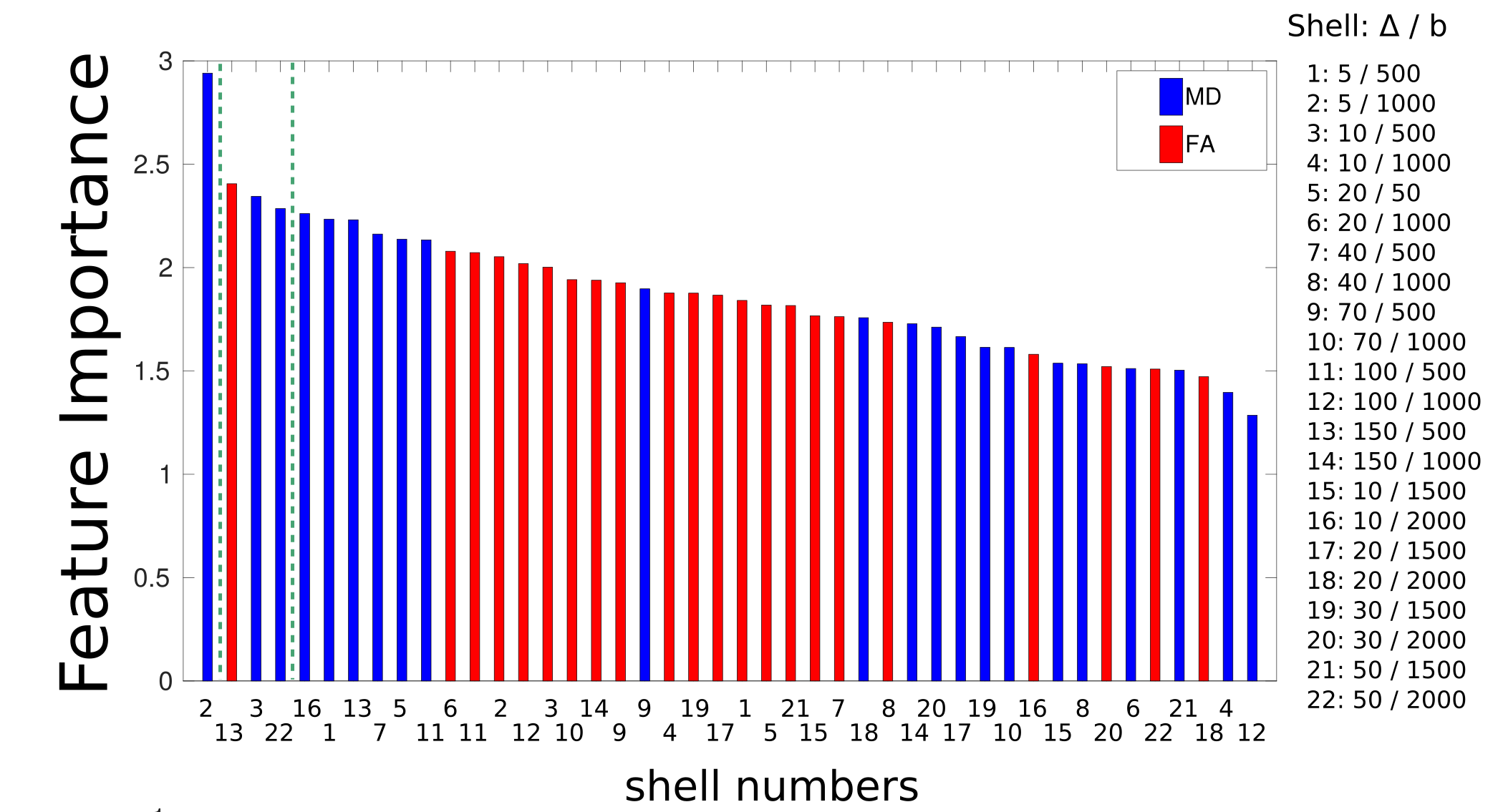
Figure 3 plots the feature importance obtained from the RF classification. The most informative feature appears to be MD measured at short diffusion time (Δ = 5ms and b=1000s/mm2).
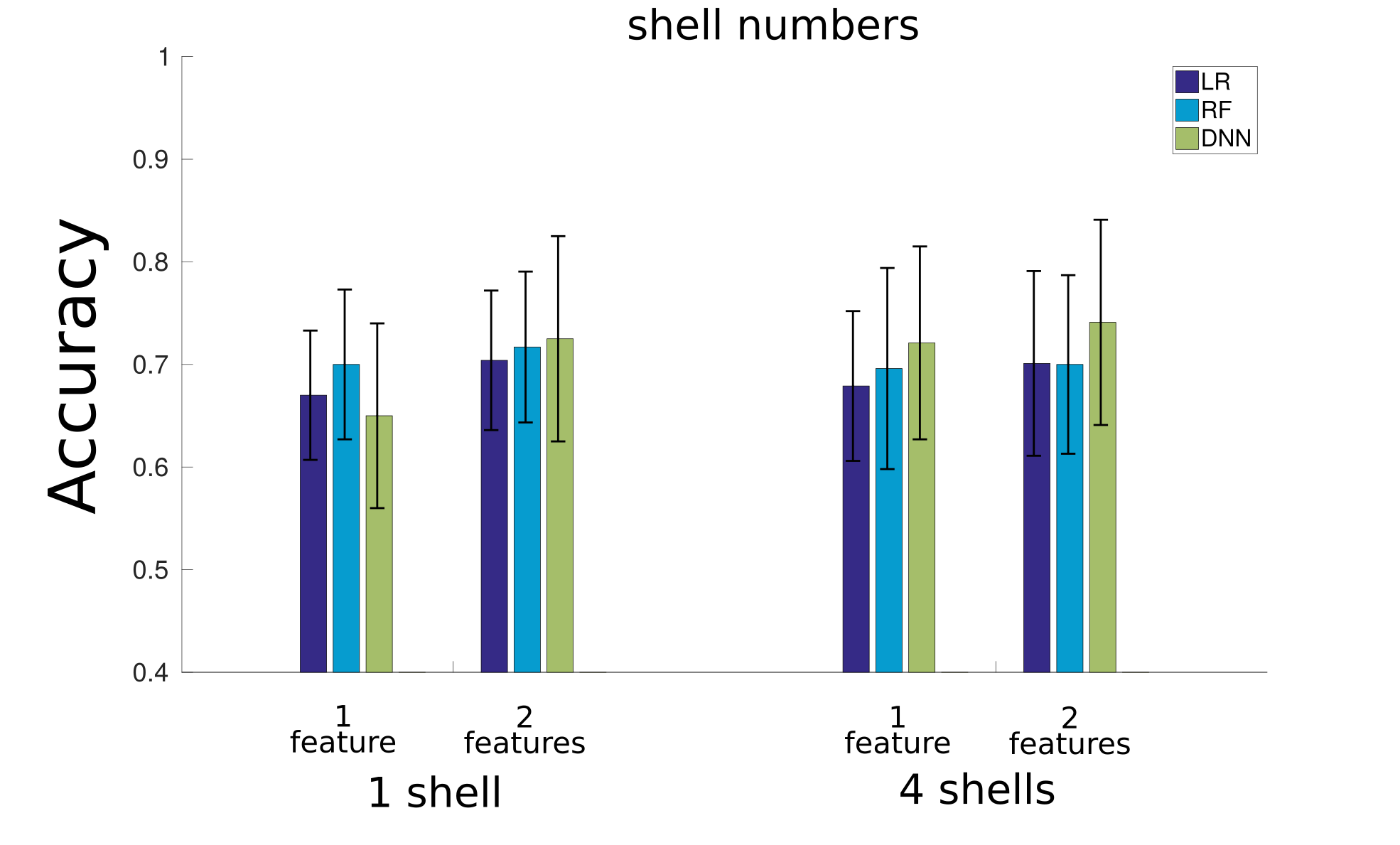
Next, we re-perform the classification for LR, RF and DNN with a reduced number of features: 1 or 4 shells with either only the best feature or both MD and FA. As illustrated in Figure 4, for 1 shell, including both MD and FA increases the accuracy for all classifiers, nevertheless, the increase is significant only for the DNN. The accuracy with reduced features is smaller than the initial values, however the difference is not significant (except for DNN with 1 shell).
Discussion
This work investigates the classification accuracy of benign and malignant lymph nodes based on dMRI data. For this dataset with 51 lymph nodes, LR, RF, DNN and CNN show similar accuracy (~75%) which is higher than previously reported values in the literature for clinical data6, with CNN exhibiting the least variability. In terms of feature importance, MD is more informative than FA and the preferred shell is acquired at short diffusion time and b = 1000s/mm2, nevertheless including both MD and FA in the classification slightly improves the accuracy. Future work will also investigate the accuracy of CNN with a reduced number of features.Acknowledgements
This study was supported by EPSRC grants EP/M020533/1 and EP/N018702/1. NS, IS and CM are supported by Champalimaud Research. DR and DCA are supported by a project that has received funding from the European Unions Horizon 2020 research and innovation programme under grant agreement number 666992.References
1 Grone, J. et al, Accuracy of Various Lymph Node Staging Criteria in Rectal Cancer with Magnetic Resonance Imaging, J Gastrointest Surg (2018) 22: 146.
2 Ogawa, M., et al, The Usefulness of Diffusion MRI in Detection of Lymph Node Metastases of Colorectal Cancer. Anticancer Research, 2016. 36(2): p. 815-9.
3 Yasui, O., et al, Diffusion-weighted imaging in the detection of lymph node metastasis in colorectal cancer. Tohoku J Exp Med, 2009. 218(3): p. 177-83.
4 Heijnen, L.A., et al., Diffusion-weighted MR imaging in primary rectal cancer staging demonstrates but does not characterise lymph nodes. Eur Radiol, 2013. 23(12): p. 3354-60.
5 Ianus, A. et al, Comparison of diffusion MR models in lymph nodes at ultra high field. ISMRM, 2018
6 Hasbahceci, M. et al, Diffusion MRI on lymph node staging of gastric adenocarcinoma, Quant Imaging Med Surg. 2015 Jun; 5(3): 392–400.
Figures