4792

Convolutional Neural Network for Real-Time High Spatial Resolution Functional Magnetic Resonance Imaging

Cagan Alkan¹, Zhongnan Fang², and Jin Hyung Lee^1,3,4,5

¹Electrical Engineering, Stanford University, Stanford, CA, United States, ²LVIS Corporation, Palo Alto, CA, United States, ³Neurology, Stanford University, Stanford, CA, United States, ⁴Bioengineering, Stanford University, Stanford, CA, United States, ⁵Neurosurgery, Stanford University, Stanford, CA, United States

Synopsis

We propose a convolutional neural network (CNN) based real-time high spatial resolution fMRI method that can reconstruct a 3D volumetric image (140x140x28 matrix size) in 150 ms. We achieved 4x spatial resolution improvement using variable density spiral (VDS) trajectory design. The proposed method achieves similar reconstruction performance as our earlier compressed sensing reconstructions while achieving 17x faster reconstruction time. We demonstrate that this method accurately detects cortical layer specific activity.

Introduction

High-resolution fMRI can enable investigation of cortical layers and sub-nuclei specific brain function. However, acquiring high-resolution MRI images can be prohibitively long. One possible approach to achieving high resolution without increasing the scan time is collecting under sampled data in combination with non-linear reconstruction methods. Compressed sensing methods^1,2 have been developed for this task, but the iterative nature of CS reconstruction makes its utilization in real-time fMRI difficult. In this study, we propose a transfer learning based convolutional neural network (CNN) approach that achieves 4x spatial resolution improvement over a fully-sampled acquisition with the same echo and acquisition time with a 3D reconstruction time of 150 ms.

Methods

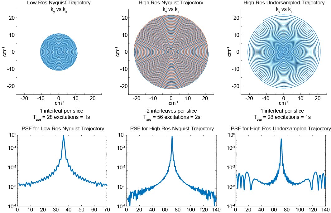
We designed a multi-slice 2D CNN fMRI trajectory using a variable density spiral (VDS) design. In our VDS design, sampling density in k-space is controlled by varying the effective field of view ($$$FOV_e$$$) as a function of $$$k_r$$$

$${FOV}_e(k_r) = {FOV}_0 \exp\left(-\left(\frac{k_r}{\alpha}\right)^2\right)$$

where $$$\alpha^2$$$ adjusts the variance of $$$FOV_e$$$. For a temporal resolution of 1 s, an echo time of 16 ms, we first designed a fully sampled trajectory with 32 mm x 32 mm FOV and the highest possible spatial resolution: 0.457 mm x 0.457 mm. Then, based on the VDS method, we designed the real-time CNN trajectory with the same FOV, temporal resolution and echo time but with 4 times higher in-plane resolution (0.229 mm x 0.229 mm). Our trajectory design is shown in Fig. 1.

Since our trajectory is under sampled, images reconstructed by gridding contain aliasing artifacts. We used a CNN approach to find the mapping between the images with aliasing artifacts and aliasing-free images. As shown in Fig. 2, 3D U-Net architecture with residual connections was used for this image-to-image transformation problem^3,4. Since the residual connection adds the input image to the 3D U-Net output, the U-Net portion of the network learns the aliasing artifact pattern to reconstruct the aliasing-free image. Gradient descent with Adam method was performed on mean squared error loss function for network training.

We first trained the network on our dataset consisting of 20 functional rat brain scans (each having 600 or 480 frames) with BOLD contrast obtained from a 7 T Bruker scanner (FOV = 32x32 mm2, matrix size = 70x70). The total number of 3D images is 10980. We interpolated the images by a factor of two at every slice to form 140x140 ground truth images. 80 % of these scans were used for training the network, and the 15 % were used for validating the training process. Then, using transfer learning, we fine-tuned the network weights on a smaller set containing 160 fully-sampled high resolution images (FOV=32x32 mm2, matrix size=140x140). Aliased input images, i.e. gridded images, are obtained by applying non-uniform FFT (nuFFT) and adjoint nuFFT operations consecutively on ground truth images. Training and model fitting were performed in Python using Keras with a TensorFlow backend. It took 22 hours to train the network for 50 epochs on 2 GeForce GTX TITAN X graphics processors. Fine-tuning the network for 50 epochs took an hour.

Experiments and Results

We compared CNN fMRI reconstruction performance with a compressed sensing (CS) reconstruction. GPU implementation of Fast Iterative Shrinkage Thresholding Algorithm (FISTA)5 was used as the baseline CS reconstruction. On average, CNN reconstruction takes 150 ms to reconstruct a volumetric 140x140x28 image, whereas CS reconstruction takes 2.6 s. Figure 3 shows example reconstruction results. Both CS and CNN reconstructions successfully remove aliasing artifacts caused by under sampling.

We evaluated the spatial resolution performance of the proposed system with simulated phantoms containing layer specific activity. As shown in Fig. 4, two interleaved layers consisting of distinct peak HRF amplitudes (2 % and 4 %, Fig. 4a) and distinct HRF shapes (Fig. 4b) were designed. We found that CNN fMRI and CS reconstruction successfully resolves different layers in both cases, while Nyquist sampled highest spatial resolution image fails to do so.

Discussion and Conclusions

We demonstrated a convolutional neural network based high spatial resolution fMRI reconstruction method that can reconstruct a 3D volumetric image (140x140x28 matrix size) in 150 ms. Experiments requiring higher spatial resolutions can benefit from the proposed method with the 4 times spatial resolution improvement. Real-time nature of the method makes it a useful tool for future studies with real-time feedback control. In summary, the proposed CNN-based real-time high-resolution CS fMRI offers an important tool to the advancement of fMRI technology.

Acknowledgements

This work was supported by NIH/NIA RF1AG047666, NIH/NINDS R01NS087159, NIH/NINDS R01NS091461, and NIH/NIMH RF1MH114227.

References

1. Fang, Z., Van Le, N., Choy, M., & Lee, J. H. (2016). High spatial resolution compressed sensing (HSPARSE) functional MRI. Magnetic resonance in medicine, 76(2), 440-455.

2. Zong, X., Lee, J., Poplawsky, A. J., Kim, S. G., & Ye, J. C. (2014). Compressed sensing fMRI using gradient-recalled echo and EPI sequences. NeuroImage, 92, 312-321.

3. Lee, D., Yoo, J. & Ye, J. C. Deep residual learning for compressed sensing MRI. in 2017 IEEE 14th International Symposium on Biomedical Imaging (ISBI 2017) 15–18 (IEEE, 2017). doi:10.1109/ISBI.2017.7950457

4. Ronneberger O et al. U-net: Convolutional networks for biomedical image segmentation, MICCAI, 2015;234-241

5. Beck, Amir, and Marc Teboulle. A fast iterative shrinkage-thresholding algorithm for linear inverse problems. SIAM journal on imaging sciences 2.1 (2009): 183-202.

Figures

Figure 1. Low resolution Nyquist, high resolution Nyquist and high resolution undersampled trajectories (top) and corresponding point spread functions (bottom) for BOLD fMRI with 16 ms echo time.

Figure 2. 3D U-Net with residual connection was used as the network architecture for reconstruction. The network maps aliased magnitude images to aliasing-free magnitude images. It consists of three-dimensional convolutional, max-pooling, transpose convolutional and concatenation layers. Batch normalization is applied after the ReLU activation function. The architecture contains 5 levels with different resolutions. Since the residual connection adds the input image to 3D U-Net output, 3D U-Net learns the residual the between ground truth and aliased images, which is the aliasing artifact pattern generates by the under sampled trajectory.

Figure 3. Reconstruction error on a sample slice.Reconstruction error on a sample slice. Top row shows a sample slice from a 3D ground truth image and gridding, compressed sensing, and convolutional neural network reconstructions from the undersampled k-space representation of ground truth image. The bottom row shows 10 times magnified errors between the sample slice and each of the reconstructions. CS and CNN methods successfully remove most of the aliasing artifacts caused by under sampling.

Figure 4. Real-time high-resolution CNN fMRI resolves layer specific activity. A phantom that is challenging to reconstruct with low spatial resolution was designed with an interleaved pattern consisting of distinct peak HRF amplitude (a) and HRF shape (b). Nyquist acquisition fails to separate the layered pattern in both cases. In contrast, CS and CNN reconstructions successfully resolve the layered patterns. Because the amplitude reduction on CNN reconstructed HRFs is smaller, CNN reconstructed amplitude map matches the ground truth map better than iterative CS reconstruction.

Proc. Intl. Soc. Mag. Reson. Med. 27 (2019)

4792