4789
A New Deep Learning Structure for Improving Image Quality of a Low-field Portable MRI System1Engineering Product Development, Singapore University of Technology and Design, SINGAPORE, Singapore, 2Information Systems Technology and Design, Singapore University of Technology and Design, SINGAPORE, Singapore, 3Centre for Medical Image Computing and Dept. Computer Science, UCL, London, United Kingdom, 4Center for Frontier Medical Engineering, Chiba University, Chiba, Japan, 5Department of Surgery, National University of Singapore, Singapore, Singapore
Synopsis
A permanent magnet based low-field MRI system provides portability and affordability. However, the quality of the image is low due to a low signal-to-noise ratio (SNR). We propose a new deep learning structure which effectively integrates denoising-networks end-to-end to super-resolution-networks, to transfer the rich information available from one-off experimental imaging from a mid-field MRI scanner (1.5T) to the lower-quality data from a portable system. The procedure uses matched pairs to learn mappings from low-quality to the corresponding high-quality images. Using the proposed method, the quality and resolution of an image from a low-field MRI system is significantly improved.
INTRODUCTION
Low-field MRI systems using permanent magnet arrays offer portability with affordability[1-2]. However, the field strength is relatively low which results in a low signal-to-noise ratio (SNR), and thus a low image quality. Here, we propose a new deep learning structure, which effectively integrates denoising-networks end-to-end to super-resolution-networks, to transfer the rich information available from one-off experimental imaging from mid-field MRI scanners (1.5T) to the lower-quality data from portable systems. We propose to use matched pairs to learn mappings from low-quality to the corresponding high-quality images.
Deep-neural-network(DNN) has been applied to single-image super-resolution[3-9]. A direct application of super-resolution on noisy images leads to inevitable magnified noises and distortions. Denoising is necessary before super-resolving images. In[10], convolutional-neural-network(CNN) was used to yield residuals, obtaining superior performance over other denoisers. End-to-end networks for jointly denoising and super-resolution were applied to restore natural images[11]. However, they are complexed and computationally expensive. For MRI images, the diversity between an image-pair is low, and it allows multiple scans of the same subject. The available networks are unnecessarily complicated, which could result in non-convergence or overfitting to training data.
MATERIALS & METHODS
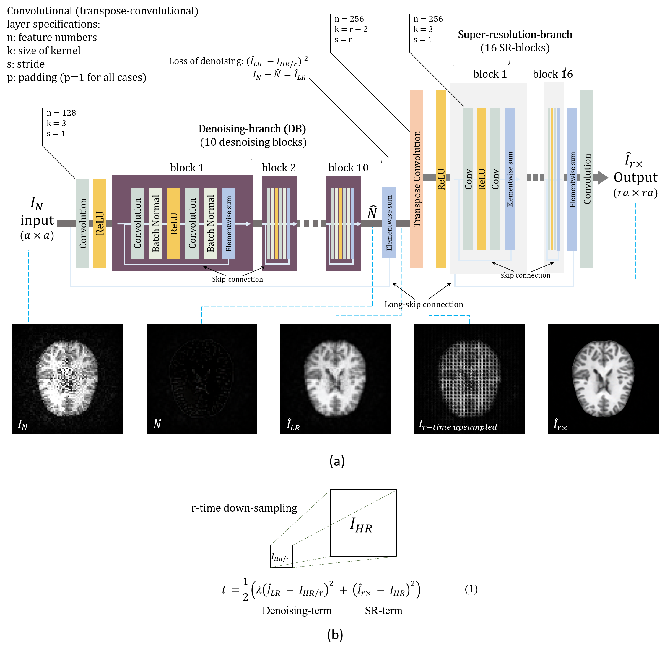
We propose a simpler and more targeted model (shown in Fig.1(a)) for a quality transformation of low-field MRI images. It consists of a denoising-branch with 10 denoising-blocks and a super-resolution-branch with 16 super-resolution-blocks, bridged by a transpose-convolutional-layer. The number of parameters is half of that of EDSR[9]. A loss function in (1) (Fig.1(b)) which consists of a denoising-term and a super-resolution-term was used to drive the learning. Term-1 is the weighted difference of the low-resolution noise-free-image, $$$\hat{I}_{LR}$$$ ($$$\hat{I}_{LR}=I_N-\hat{N}$$$, at the exit of denoising-branch), and the $$$r$$$-time down-sampled high-quality image, $$$I_{HR/r}$$$.
In Fig.1(a), each denoising-branch consists of two convolutions, two batch-normalization, an activation function (rectified-linear-unit (ReLU)), and an element-wise summation, with the size of convolution kernel, stride, and padding labeled. Instead of explicitly calculating the noise-residual of images[10], a long skip-connection was used as the residual-yielding-process internally to obtain $$$\hat{I}_{LR}$$$. Thus, the networks can be trained through Term-1 in (1) using intermedium-predicted images rather than noise patterns. In Fig.1(a), following the denoising-branch, transpose-convolutional-layer up-samples the matrix $$$r$$$-time for further super-revolving. The super-resolution-branch is similar to the denoising-branch without batch-normalization because batch-normalization does not favor super-resolving fine features or maintain original contrast levels[9]. Skip-connection was applied to this branch. Super-resolution-branch outputs $$$\hat{I}_{r\times}$$$ and the difference between $$$\hat{I}_{r\times}$$$ and the high-quality image, $$$\hat{I}_{HR}$$$, forms Term-2 in (1).
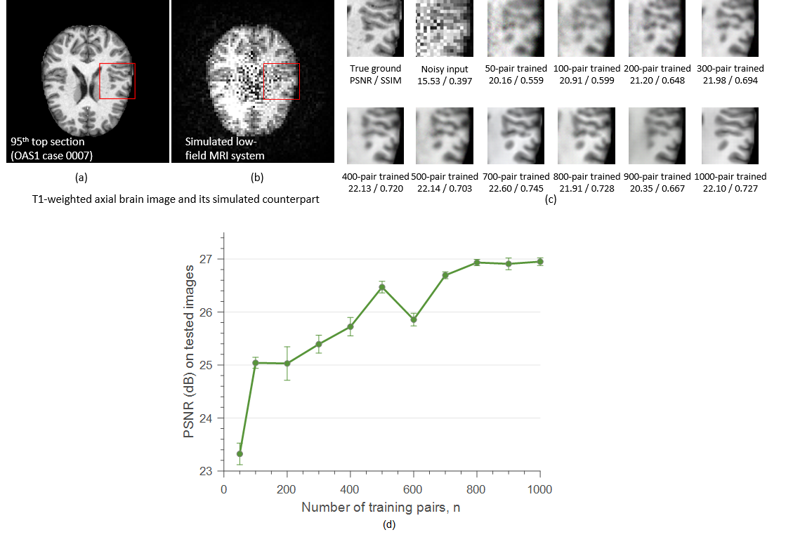
To train the network, 1000 high-quality images (1.5T, Siemens, $$$240\times 240$$$pixels) were downloaded[12] and the corresponding low-field low-quality images were generated based on the Halbach-array-based low-field MRI system (68mT)[2]. An encoding term, $$$C_q(\mathbf{r})e^{-i2\pi\gamma\mathbf{B_0}t}$$$, was used from the signal equation $$$S_q(t)=\int_VC_q(\mathbf{r})e^{-i2\pi\gamma\mathbf{B_0}t}m(\mathbf{r})d\mathbf{r}$$$ to generate low-field images where $$$C_q(\mathbf{r})$$$ is the sensitivity of the $$$q^{th}$$$ coil, $$$\mathbf{B_0}$$$ is the spatial encoding magnetic field. The resolution of the image is determined by the pattern of $$$\mathbf{B_0}$$$[13]. It is down-sampled $$$r$$$-time. Gaussian-white-noise with a deviation of $$$\sigma_\textrm{sigma}$$$ was added to the signal to obtain noisy images. When $$$\sigma_\textrm{sigma}=-20$$$dB, the standard deviation of the noise-residual-image ($$$\sigma$$$) is 0.1. Both the high-quality images (Fig.2(a)) and the noisy low-resolution ones (Fig.2(b)) from the low-field system were fed to the network for training.
RESULTS
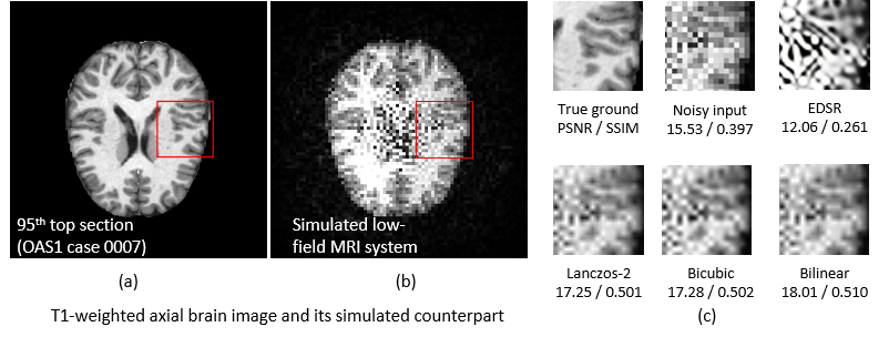
Peak-SNR(PSNR) and structure-similarity-index(SSIM) were used to evaluate the quality of the reconstructed images. Fig.2(c) shows the reconstructed images using different numbers of training pairs ($$$n$$$) and Fig.2(d) shows the average PSNR of the tested images ($$$\sigma=0.1$$$) versus $$$n$$$. As shown, the quality and resolution of the images are significantly improved by the proposed network when it is trained sufficiently. The PSNR and SSIM are about 22 and 0.700, respectively when $$$n=700$$$, which takes approximately two hours (GPU: $$$4\times11$$$GB NVIDIA GTX1080Ti). Moreover, Fig.3 shows the reconstructed images with super-resolution without denoising. As shown, super-resolution does not suppress the noise of the images but introducing distortions.DISCUSSION & CONCLUSION
Here, a deep learning structure, which is an end-to-end effective integration of denoising-networks and super-resolution-deep-networks, is proposed to transfer low-quality noisy images from a low-field system to high-quality images. It is successfully demonstrated using simulated data from a Halbach-array-based low-field MRI system. Next, scanned images will be used to test the proposed technique where practical situations, e.g. real noise and a relative location mismatch between the images in a pair, will be taken into consideration.Acknowledgements
Singapore MIT Alliance Research and Technology (SMART) innovation grant (ING137068-BIO)References
1. C.Z. Cooley, J.P. Stockmann, B.D. Armstrong, M. Sarracanie, M.H. Lev, M.S. Rosen, et al. Two-dimensional imaging in a lightweight portable MRI scanner without gradient coils Magn. Reson. Med, 73 (2015), pp. 872-8832. 2. Z.H. Ren, S. Obruchkov, D.W. Lu, R. Dykstra, S.Y. Huang. A low-field portable magnetic resonance imaging system for head imaging. In Progress in Electromagnetics Research Symposium-Fall (PIERS-FALL), 2017 2017 Nov 19 (pp. 3042-3044). 3. D.C. Alexander, D. Zikic, A. Ghosh, R. Tanno, V. Wottschel, J. Zhang, E. Kaden, T.B. Dyrby, S.N. Sotiropoulos, H. Zhang, A. Criminisi Image quality transfer and applications in diffusion MRI Neuroimage, 152 (2017), pp. 283-298, 10.1016/j.neuroimage.2017.02.089 4. R. Tanno, D. E. Worrall, A. Ghosh, E. Kaden, S. N. Sotiropoulos, A. Criminisi, Daniel C. Alexander, Bayesian Image Quality Transfer with CNNs: Exploring Uncertainty in dMRI Super-Resolution, Springer International Publishing 2017 5. Y. LeCun, Y. Bengio, and G. Hinton. Deep learning. Nature, 521(7553):436–444, May 2015. 6. C. Dong, C. C. Loy, K. He, and X. Tang. Learning a Deep Convolutional Network for Image Super-Resolution. In European Conference on Computer Vision (ECCV), pages 184–199, 2014. 7. J. Kim, J. K. Lee, and K. M. Lee. Accurate image superresolution using very deep convolutional networks. In IEEE Conference on Computer Vision and Pattern Recognition (CVPR), pages 1646–1654, 2016. 8. C. Ledig, L. Theis, F. Huszar, J. Caballero, A. Cunningham, A. Acosta, A. P. Aitken, A. Tejani, J. Totz, Z. Wang, and W. Shi. Photo-Realistic Single Image Super-Resolution Using a Generative Adversarial Network. In IEEE Conference on Computer Vision and Pattern Recognition (CVPR), pages 105–114, 2017. 9. B. Lim, S. Son, H. Kim, S. Nah, and K. M. Lee., Enhanced Deep Residual Networks for Single Image Super-Resolution, 2017 IEEE Conference on Computer Vision and Pattern Recognition Workshops (CVPRW), Honolulu, HI, 2017, pp. 1132-1140, doi: 10.1109/CVPRW.2017.151 10. K. Zhang, W. Zuo, S. Gu, and L. Zhang. Learning Deep CNN Denoiser Prior for Image Restoration. In IEEE Conference on Computer Vision and Pattern Recognition (CVPR), pages 3929–3938, 2017. 11. D Park, K Kim, SY Chun Efficient Module Based Single Image Super Resolution for Multiple Problems. In IEEE Conference on Computer Vision and Pattern Recognition (CVPR), pages 995-1003, 2018. 12. D. S. Wang, T. H. Parker, J. Csernansky, J. G. Morris, J. C. Buckner, R. L. Open Access Series of Imaging Studies (OASIS): Cross-Sectional MRI Data in Young, Middle Aged, Nondemented, and Demented Older Adults Marcus, Journal of Cognitive Neuroscience, 19, 1498-1507. doi: 10.1162/jocn.2007.19.9.1498 13. G Schultz, H Weber, D Gallichan, WRT Witschey, AM Welz, CA Cocosco, J Hennig, M Zaitsev. Radial imaging with multipolar magnetic encoding fields. IEEE Trans Med Imaging 2011;30:2134–2145Figures