Synopsis

There has been an increasing interest for systems that combine a linear accelerator with a MRI. The goal of such systems is to allow for real-time adaptive radiotherapy; to have the ability to track a region of interest for the purpose of accurate radiation delivery. This requires the ability to image in real-time. We investigated the use of convolution neural networks (CNNs) for the purpose of real-time imaging. The reconstruction time of our preliminary data was 150 ms using a NVIDIA 1080Ti GTX GPU. Further optimization of the CNN parameters may decrease the reconstruction time below 100 ms.

INTRODUCTION:

With recent advances in systems combining MRI with a linear accelerator (Linac-MR), real-time MRI is becoming an increasingly important requirement for adaptive radiotherapy.^1-4 In order to utilize Linac-MR systems for real-time adaptive radiotherapy, real-time MRI techniques are required to track tumor and/or organs of interest. Convolutional neural networks (CNN's) have become increasingly popular given the accessibility of GPU's and code repositories specifically designed for CNN's. Our study investigated real-time CNN reconstruction using retrospectively and prospectively undersampled MR data.

METHODS:

Data Acquisition

Data was acquired using our 3T Philips Achieva system (Philips Medical Systems, Cleveland, OH, USA). Both the retrospective and prospective data was acquired using a bSSFP sequence (TR/TE=2.2/1.1 ms) at a FOV of 40x40 cm², slice thickness of 2 cm, and flip angle of 20^o. Undersampling was achieved using a dynamic incoherent sampling pattern, similarly to those used for compressed sensing. The prospective undersampling required a patch that we developed for our Philips system. Our retrospective data consisted of six non-small cell lung tumor patients. For each patient we acquired 650 dynamic frames. For the prospectively undersampled motion phantom data, we acquired fully sampled data (to train our CNN), as well as data at 4x acceleration.

Convolution Neural Network

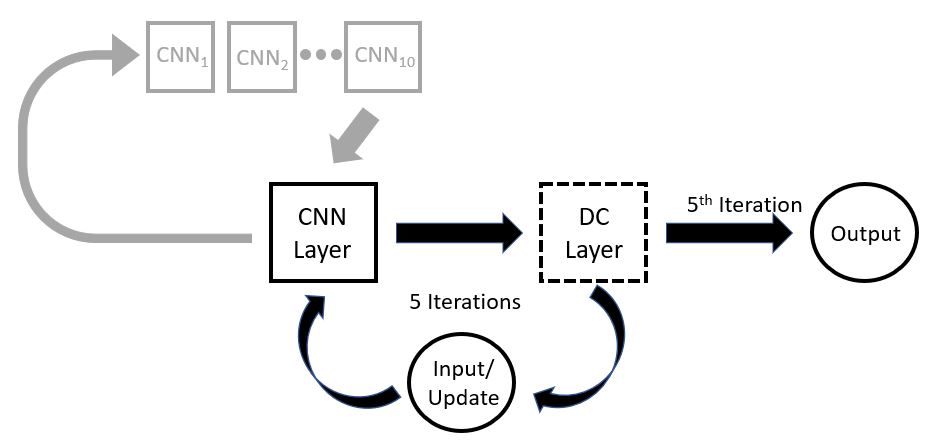
The real-time CNN reconstruction code we developed is displayed in Figure 1 and was based on the recent study by Schlemper et al. that we modified for real-time reconstruction.⁵ The retrospective patient data was trained using the first 250 dynamics at 5x and 10x undersampling rates for each patient separately, resulting in a network optimized to each patient’s motion. The prospective phantom data was trained at a 4x undersampling rate. Each network was initially trained at a coarse learning rate, which was then fed into a fine-tuning step, with a smaller optimization step size.

A quantitative analysis was conducted on the retrospective data. The Dice coefficient (DC) of the segmented tumor structure was computed, comparing the segmentation ability of the CNN reconstruction to the fully sampled images, to investigate the CNN reconstruction on small structures of interest.⁶ The normalized mean square error (NMSE) was computed to investigate artifacts produced in the CNN reconstruction. The total training time took 2 hours using a single NVIDIA 1080Ti GTX GPU.

RESULTS:

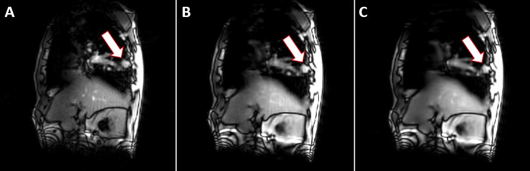
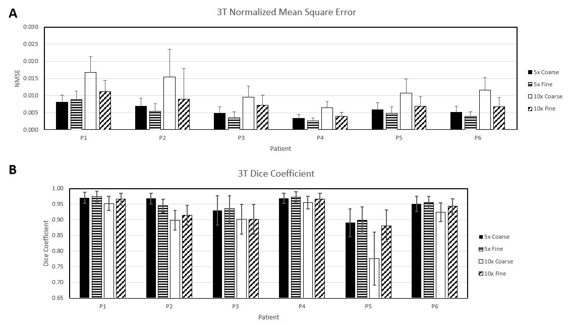
An example of the retrospective CNN reconstruction is shown in Figure 2. For each data set and each tuning step, the DC and NMSE was calculated for each dynamic frame. Figure 3A contains the NMSE for each of the patient data, at 5x and 10x acceleration for each coarse and fine tuning step. Figure 3B contains a plot of the DC results values averaged over 400 frames from the CNN reconstructed data for each patient. With the exception of patient 5, every patient had a DC above 0.9. Patient 5 had an irregular tumor shape, resulting in a reduced DC.

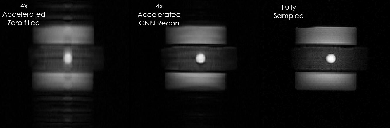
The qualitative prospective CNN results for our motion phantom acquired at 4x acceleration is shown in Figure 4. It is evident that the artifacts have been greatly reduced. Furthermore, it can be seen that the CNN reconstruction was able to reproduce the phantom edges, and spherical shape of the central fiducial.

The reconstruction time for the CNN reconstruction for both the retrospective and prospective data was 150 ms.

DISCUSSION:

The total training time for the coarse and fine tuning stages took 1 hour each, for a total training time of 2 hours. The reconstruction time per image was 150 ms using a NVIDIA 1080Ti GTX GPU. Increasing the training time will increase the quality of images, which we intend to investigate. While the CNN reconstruction provided qualitatively and quantitatively excellent images, we are still optimizing the parameters to further increase the image quality and decrease the reconstruction time. Furthermore, we did not implement any data augmentation within our training data. Data augmentation can be used to increase amount of training data by introducing minor shifts and warps to the training data, making the network more robust.

We believe with careful tuning of the CNN parameters that we can achieve reconstruction times well below 100 ms.

CONCLUSION:

Acknowledgements

We would like to acknowledge our funding source: Alberta Innovates CRIO Team Grant.

We would also like to acknowledge Philips Medical Systems for research support.

References

1. B.G Fallone, B Murray, S Rathee, et al. First MR images obtained during mega-voltage photon irradiation from a integrated linac-MR system. Med Phys. 2009;36:2084-2088.

2. PJ Keall, M Barton, and S Crozier. The Australian magnetic resonance imaging-linac program. Radiother Oncol. 2014;24:203-206.

3. BW Raaymakers, JJ Lagendijk, J Overweg, et al. Integrating a 1.5 T MRI scanner with a 6 MV accelerator: proof of concept. Phys Med Biol. 2009;54:N229-N237.

4. S Mutic and JF Dempsey. The Viewray system: magnetic resonance guided and controlled radiotherapy. Semin Radiat Oncol. 2014;24:196-199.

5. J Schlemper, J Caballero, JV Hajnal, AN Price, and D Rueckert. A deep cascade of convolutional neural networks for dynamic MR image reconstruction. IEEE Trans on Med Imaging;37:491-503.

6. J Yun, E Yip, Z Gabos, et al. Improved lung tumor autocontouring algorithm for intrafractional tumor tracking using 0.5 T Linac-MR. Biomed Phys Eng Express. 2016;2:1-5.