4776
Fidelity Imposing Network Edit (FINE) for Solving Ill-Posed Image Reconstruction1Department of Biomedical Engineering, Cornell University, Ithaca, NY, United States, 2Department of Radiology, Weill Medical College of Cornell University, New York, NY, United States, 3Department of Electrical and Computer Engineering, Cornell University, Ithaca, NY, United States
Synopsis
A Fidelity Imposing Network Edit (FINE) method is proposed for solving inverse problem that edits a pre-trained network's weights with the physical forward model for the test data to overcome the breakdown of deep learning (DL) based image reconstructions when the test data significantly deviates from the training data. FINE is applied to two important inverse problems in neuroimaging: quantitative susceptibility mapping (QSM) and undersampled multi-contrast reconstruction in MRI.
Introduction
DL-based image reconstruction approaches typically establish network weights using supervised learning and may not perform well on a test data that deviates from the training data(1). This is because these DL-based techniques are often agnostic about the physical model of signal generation or data fidelity underlying image systems. The data fidelity may be imposed in Bayesian inference involving explicit image feature extractions that may forfeit some DL benefits. Here, we propose to embed deeply data fidelity into all layers in the network by editing a pre-trained network's weights through backpropagation according to the fidelity of a test data, and we refer to this method as Fidelity Imposing Network Edit (FINE).Methods
FINE is applied to two important inverse problems in neuroimaging: quantitative susceptibility mapping (QSM) and undersampled multi-contrast reconstruction in MRI.
Data acquisition and processing:
For QSM, we obtained 6 healthy subjects, 8 patients with multiple sclerosis (MS) and 8 patients with intracerebral hemorrhage (ICH), with $$$256\times256\times48$$$ matrix size and $$$1\times1\times3mm^3$$$ resolution. MRI was repeated at 5 different orientations per healthy subject for COSMOS reconstruction(2), which was used as the gold standard for brain QSM. For multi-contrast reconstruction, we obtained and co-registered T1w, T2w, and T2FLAIR axial images of 237 patients with MS diseases, with $$$256\times176$$$ matrix size and $$$1mm^3$$$ isotropic resolution.
Supervised Training:
For QSM, we implemented a dipole inversion network using a 3D U-Net(3,4) $$$\phi(;\Theta)$$$ with weights $$$\Theta$$$ for mapping from local tissue field $$$f$$$ to COSMOS QSM $$$\chi$$$. Five of the 6 healthy subjects were used for training, giving a total number of 12025 $$$64\times64\times16$$$ patches, in which $$$20%$$$ were selected randomly as validation set. We employed the same combination of loss function as in (4) in training the network with Adam optimizer(5) (learning rate 0.001, epoch 40), resulting a 3D U-Net $$$\phi(;\Theta_0)$$$.
For multi-contrast reconstruction, we employed a 2D U-Net(6) $$$\phi(;\Theta)$$$ with weights $$$\Theta$$$ for mapping from a fully sampled T1w image $$$v$$$ to a fully sampled T2w image $$$u$$$. 8800/2200/850 slices were extracted from multi-contrast MS dataset as the training/validation/test dataset. We used the L1 difference between the network output and target image as the loss function in training the network with Adam(5) (learning 0.001, epoch 40), resulting a 2D U-Net $$$\phi(;\Theta_0)$$$. A similar 2D U-Net was established for T2FLAIR images.
Fidelity Imposing Network Edit (FINE):
For QSM, given a new local field $$$f$$$, the network weights $$$\Theta_0$$$ from supervised training was used to initialize the weights $$$\Theta$$$ in the following minimization: $$\hat{\Theta} = \arg\min_{\Theta}||W(d*\phi(f;\Theta)-f) ||^2_2$$where $$$W$$$ the noise weighting, $$$d$$$ the dipole kernel.
For multi-contrast reconstruction, given undersampled axial T2w k-space data $$$b$$$ and corresponding fully-sampled T1w image $$$v$$$, the network weights $$$\Theta_0$$$ from supervised training was used to initialize the weights $$$\Theta$$$ in the following minimization: $$\hat{\Theta} = \arg\min_{\Theta}||UF\phi(v;\Theta)-b||^2_2$$where $$$U$$$ the binary random variable density k-space under-sampling mask, $$$F$$$ the Fourier Transform operator.
Above equations were solved using Adam(5) (learning rate 0.001, iterations stop when relative decrease of the loss function between two consecutive epochs reached 0.01). The final reconstruction of the edited network was $$$\hat{\chi}=\phi(f;\hat{\Theta})$$$ for QSM and $$$\hat{u}=\phi(v;\hat{\Theta})$$$ for T2w image. Similarly, T2FLAIR images were reconstructed.
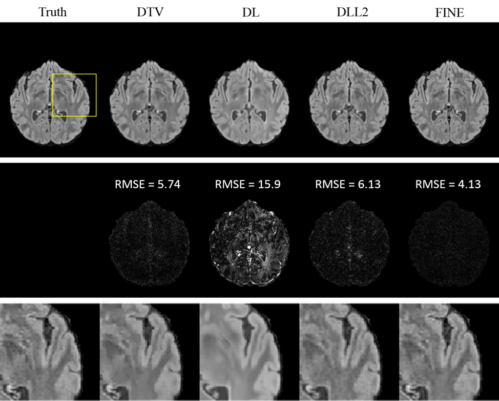
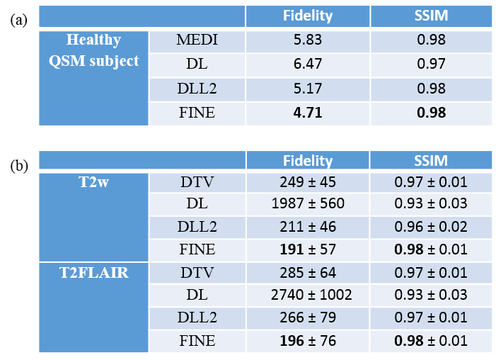
For comparison, total variation regularization (MEDI(7) in QSM, DTV(8) in multi-contrast reconstruction), Supervised Training (DL), DL based L2 regularization (DLL2) were used. The fidelity cost ( $$$||W(d*\chi-f) ||_2$$$ in QSM, $$$||UFu-b||_2$$$ in multi-contrast reconstruction) and structural similarity index (SSIM)(9) were calculated for each method, with COSMOS(2) as ground truth for QSM and fully sampled T2w/T2FLAIR images as ground truth for multi-contrast reconstruction.
Results
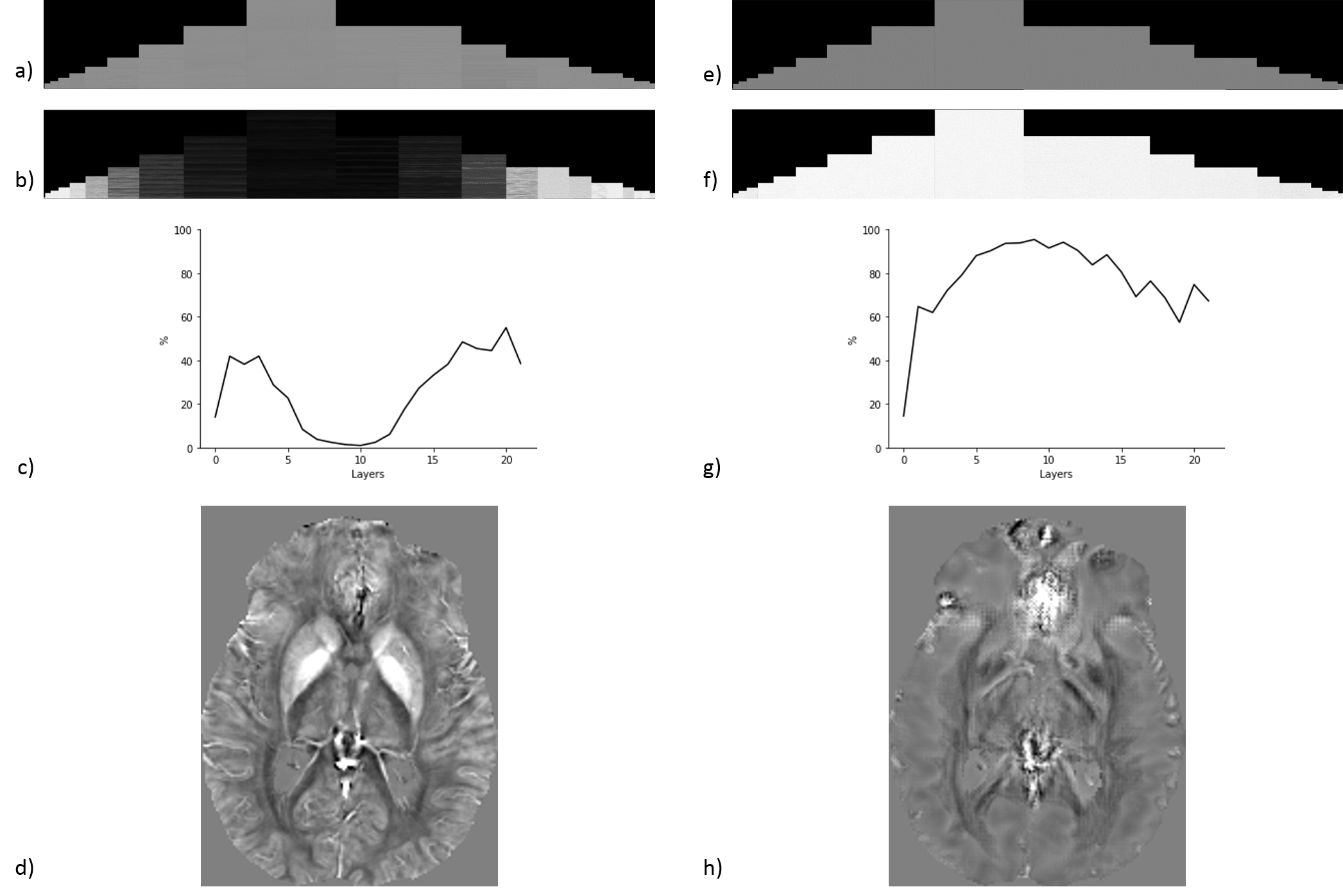
The differences between $$$\Theta_0$$$ and $$$\Theta$$$ were shown in Figure 1 applying FINE in reconstructing QSM of an MS patient. FINE changed substantially the weights only in the encoder and decoder parts of the network (Figure 1b&c). Compared to FINE, a randomized $$$\Theta$$$ initialization in above equations using a truncated normal distribution (Figure 1e) (deep image prior)(10) caused substantial changes of weights in all layers (Figure 1f&g) and resulted in markedly inferior QSM (Figure 2d&h).
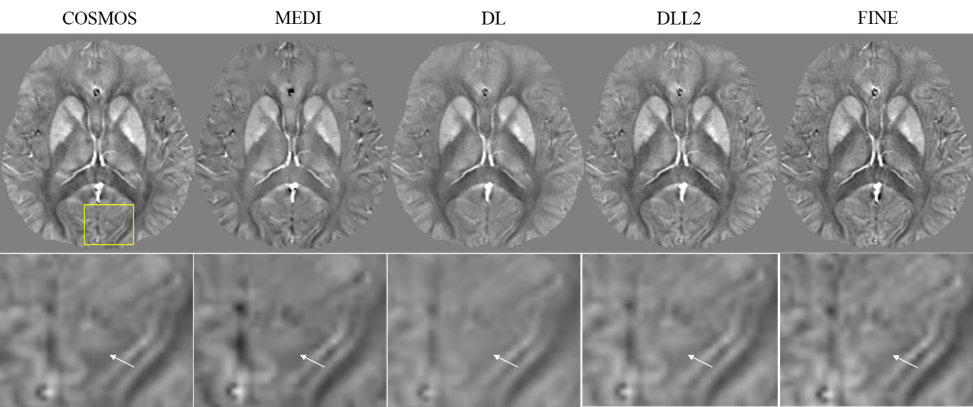
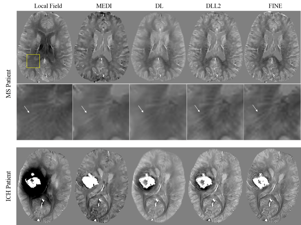
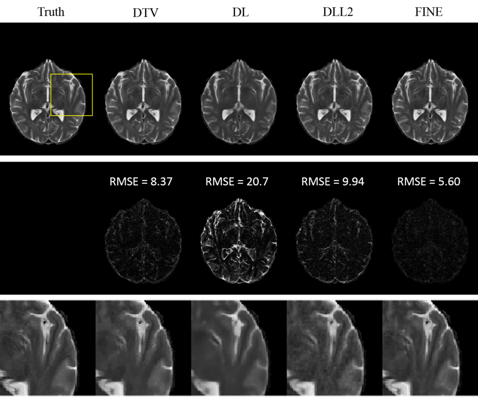
Fidelity cost and SSIM for QSM are presented in Table 1(a), those for T2w/T2FLAIR in Table 1(b). Both quantitative analysis showed superior performance of FINE compared to the other methods. For QSM, more fine structures are shown clearly in FINE for healthy subject (Figure 2) and MS patient (Figure 3), shadow artifacts were markedly suppressed in FINE for ICH patient (Figure 3). For multi-contrast reconstruction, structural details such as white/grey boundary were clearly depicted in FINE (Figure 4&5).
Discussion and conclusion
Data fidelity can be used effectively to edit deep neural network's weights on a single test data in order to produce high quality image reconstructions. This fidelity-based network edit strategy can improve performance in solving ill-posed inverse problems in medical imaging.Acknowledgements
The current work is supported by NIH grant R01 NS095562, R01 NS090464, S10 OD021782, and R01 CA181566.References
1. Suciu O, Mărginean R, Kaya Y, Daumé III H, Dumitraş T. When Does Machine Learning FAIL? Generalized Transferability for Evasion and Poisoning Attacks. arXiv preprint arXiv:180306975 2018.
2. Liu T, Spincemaille P, De Rochefort L, Kressler B, Wang Y. Calculation of susceptibility through multiple orientation sampling (COSMOS): a method for conditioning the inverse problem from measured magnetic field map to susceptibility source image in MRI. Magnetic Resonance in Medicine: An Official Journal of the International Society for Magnetic Resonance in Medicine 2009;61(1):196-204.
3. Çiçek Ö, Abdulkadir A, Lienkamp SS, Brox T, Ronneberger O. 3D U-Net: learning dense volumetric segmentation from sparse annotation. 2016. Springer. p 424-432.
4. Yoon J, Gong E, Chatnuntawech I, Bilgic B, Lee J, Jung W, Ko J, Jung H, Setsompop K, Zaharchuk G. Quantitative susceptibility mapping using deep neural network: QSMnet. NeuroImage 2018.
5. Kingma DP, Ba J. Adam: A method for stochastic optimization. arXiv preprint arXiv:14126980 2014.
6. Ronneberger O, Fischer P, Brox T. U-Net: Convolutional Networks for Biomedical Image Segmentation. Lect Notes Comput Sc 2015;9351:234-241.
7. Liu J, Liu T, de Rochefort L, Ledoux J, Khalidov I, Chen W, Tsiouris AJ, Wisnieff C, Spincemaille P, Prince MR. Morphology enabled dipole inversion for quantitative susceptibility mapping using structural consistency between the magnitude image and the susceptibility map. Neuroimage 2012;59(3):2560-2568.
8. Ehrhardt MJ, Betcke MM. Multicontrast MRI reconstruction with structure-guided total variation. SIAM Journal on Imaging Sciences 2016;9(3):1084-1106.
9. Wang Z, Bovik AC, Sheikh HR, Simoncelli EP. Image quality assessment: from error visibility to structural similarity. IEEE transactions on image processing 2004;13(4):600-612.
10. Ulyanov D, Vedaldi A, Lempitsky V. Deep image prior. arXiv preprint arXiv:171110925 2017.
Figures