4775
Learning Primal Dual Network for Fast MR Imaging1Lauterbur Research Center for Biomedical Imaging, Shenzhen Institude of Advanced Technoleoy,Chinese Academy of Sciences, Shenzhen, China, 2Department of Biomedical Engineering and Department of Electrical Engineering, University at Buffalo, The State University of New York, Buffalo, NY, United States, 3Research Center for Medical AI, Shenzhen Institude of Advanced Technoleoy, Chinese Academy of Sciences, Shenzhen, China
Synopsis
We introduce a novel deep learning network which combines elements of model and data driven approaches for fast MR imaging, termed modified Learned PD. The network is inspired by the first-order primal dual algorithm, where the convolutional neural network blocks are used to learn the proximal operators. Learned PD network works directly from undersampled k-space data and reconstructs MR images by updating in k-space and image domain alternatively. This approach has been evaluated by in vivo MR datasets and achieves accurate MR reconstructions, outperforming other comparing methods across various quantitative metrics.
Introduction
Recently, deep learning based methods have drown a lot of attentions1-6. They either learn the optimal parameters that the inverse model need or the mapping from aliased images or undersampled k-space data to clean images through a predesigned network and the training dataset. In our another work (Abstract title: Deep Chambolle-Pock Network for Accelerating MR Imaging), we have incorporated the Chambolle-Pock algorithm7, which has been successfully applied in medical image reconstruction, into a network to learn the proximal operator and parameters. In this work, we further break the structure between different variables in proximal operators and let the network freely learn the relations. The new network (named as Learned PD) was evaluated on highly undersampled in vivo MR human datasets and the experimental results show the superiority of the proposed method.Methods
The reconstruction of CS-MRI8 can be formulated as follows:$$min_p{\left\{F(Ap)+G(p)\right\}} (1)$$ where $$$ F(Ap)=||Ap-y||_2^2$$$, $$$p$$$ is the image to be reconstructed, $$$A$$$ denotes the undersampled Fourier transform, $$$y$$$ is the acquired data, $$$G(p)$$$ is a penalty function that incorporates the prior knowledge. The reconstruction problem can be solved by a first-order primal dual algorithm (also known as CP algorithm7) as following iteration: $$\begin{cases}d_{n+1}=prox_\sigma\left[F^*\right](d_n+\sigma A\overline{p}_n) \\p_{n+1}=prox_\tau\left[G\right](p_n-\tau A^*d_{n+1}) \\ \overline{p}_{n+1}=p_{n+1}+\theta(p_{n+1}-p_n) \end{cases} (2)$$ $$$\sigma$$$, $$$\tau$$$ and $$$\theta$$$ are algorithm parameters and $$$prox$$$ denotes the proximal mapping which can work directly with non-smooth objective functions. In this work, we use a Convolutional Neural Network (CNN) block to replace the proximal mapping to learn the parameterized proximal operators. The new algorithm, called Learned PD, can be formulated as: $$\begin{cases}d_{n+1}=\Gamma(d_n,Ap_n,y) \\p_{n+1}=\Lambda(p_n, A^*d_{n+1}) \end{cases} (3)$$
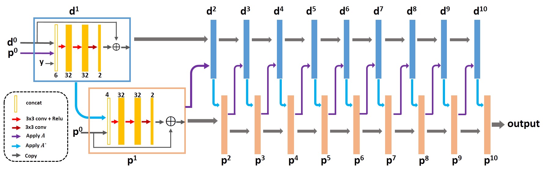
The architecture of the Learned PD is described in Figure 1. Here we further break the fixed structure between the primal and dual variables and let the network freely learn the relations. Learned PD consists of dual update and primal update. The dual and primal updates have the same structure which has 3 convolutional layers in each iteration. To train the network more easily, we made it a residual network. The convolutions are all 3x3 pixel size, and the number of channels is 4-32-32-2 for each primal update, and 6-32-32-2 for dual update where the number of outputs 2 denotes the real and imaginary parts of the data. The nonlinearities were chosen to be Rectified Linear Unites (ReLU) functions and we let the number of iterations be 10. Since each iteration involves 2 3-layer networks, the total depth of the Learned PD is 60 convolutional layers.
We validated the method using in-vivo MR datasets. Overall 200 fully sampled multi-contrast data from 2 subjects with a 3T scanner (MAGNETOM Trio, SIEMENS AG, Erlgen, Germany) were collected and informed consent was obtained from the imaging object in compliance with the IRB policy. After normalization and image augmentation through rotation and flipping, we got 1600 k-space data, where 1400 for training and 200 for validation. The model was trained and evaluated on an Ubuntu 16.04 LTS (64-bit) operating system equipped with a Tesla TITAN Xp Graphics Processing Unit (GPU, 12GB memory) in the open framework Tensorflow with CUDA and CUDNN support. We also have tested Learned PD on the data acquired from other two 3T scanners of GE (GE Healthcare, Waukesha, WI) and UIH (United Imaging Healthcare, Shanghai, China).
Results
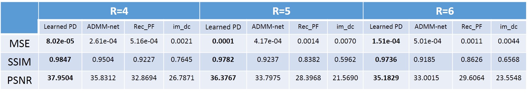
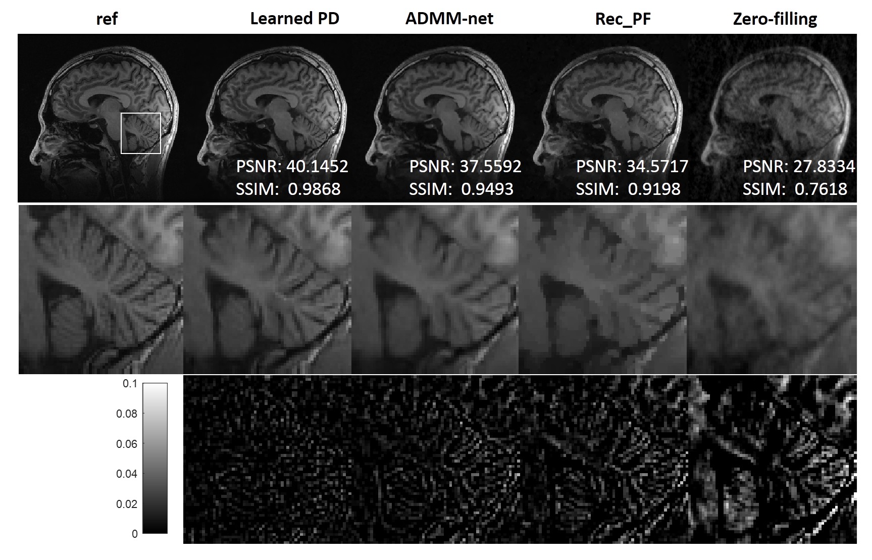
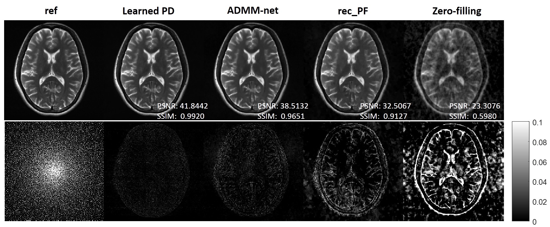
We compared the Learned PD with other CS-MRI reconstruction methods: 1) rec_PF9, traditional CSMR reconstruction method, 2) ADMM-net3, state-of-the-art model-driven CSMR reconstruction method. Several similarity metrics, including MSE, SSIM and PSNR, were used to compare the reconstruction results of different methods.
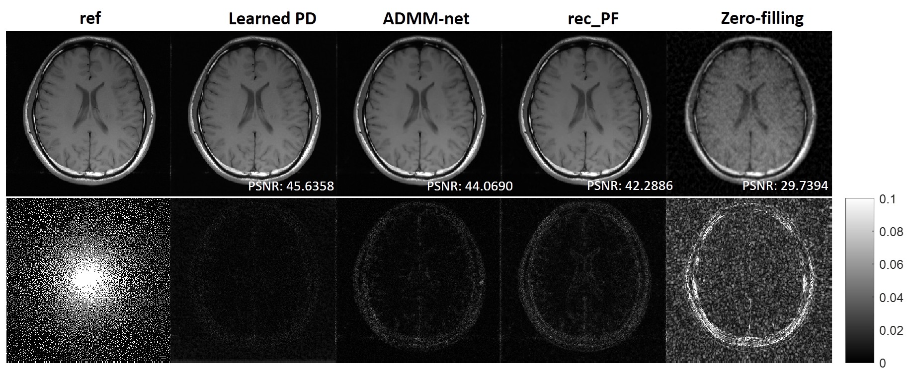
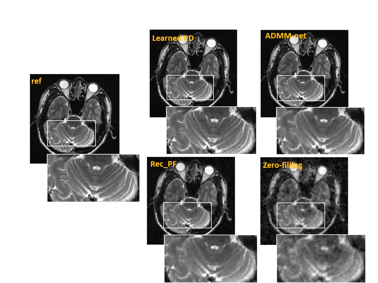
From quantitative metrics shown in Table 1, with different acceleration factors, the Learned PD all shows significant improvement over other methods. Figure 2 illustrates the reconstructions of the different methods and the corresponding error maps with acceleration factor of 4. Figure 3 and Figure 4 show the visual comparisons of different methods and the zoom-in views demonstrate the ability of the Learned PD that preserves more fine details while removing the undersampling artifacts.
Figure 5 illustrates the reconstructions of data from UIH scanner. Detailed accuracy metrics are also shown in figure.
Conclusion
We have described a new deep network for fast MR imaging in this work. The architecture of the Learned PD network is motivated by the data flow graph of the primal dual algorithm and the learned operators replace the proximal operators in original algorithm. The experimental results on in vivo data show the highly efficient reconstruction of the Learned PD in terms of both artifacts removal and detail preservation.Acknowledgements
This work was supported in part by the National Science Foundation of China (No. 61471350, No. 81729003, No. 61871373), National Science Foundation of Guangdong Province (No. 2018A0303130132), and Guangdong Provincial Key Laboratory of Medical Image Processing (No. 2017A050501026).References
1. Wang S, Su Z, Ying L, et al. Accelerating magnetic resonance imaging via deep learning. ISBI 514-517 (2016)
2. Schlemper J, Caballero J, Hajnal J V, et al. A Deep Cascade of Convolutional Neural Networks for Dynamic MR Image Reconstruction. IEEE TMI 2018; 37(2): 491-503.
3. Yang Y, Sun J, Li H, Xu Z. Deep ADMM-Net for Compressive Sensing MRI. NIPS, Barcelona, Spain, 2016.
4. Hammernik K, Klatzer T, Kobler E, et al. Learning a Variational Network for Reconstruction of Accelerated MRI Data. Magn Reson Med 2018, 79(6): 3055-3071.
5. Zhu B, Liu J Z, Cauley S F, et al. Image reconstruction by domain-transform manifold learning. Nature 2018; 555(7697): 487-492.
6. Adler J, Oktem O. Learned Primal-Dual Reconstruction. IEEE TMI 2018; 37(6): 1322-1332.
7. Chambolle A, Pock T. A First-Order Primal-Dual Algorithm for Convex Problems with Applications to Imaging. J. Math. Imag. Vis. 2011; 40:120-145.
8. Lustig M, Donoho DL, Pauly JM. Sparse MRI: The application of compressed sensing for rapid MR imaging. Magn Reson Med 2007; 58:1182–1195.
9. Yang J, Zhang Y, Yin W, et al. A Fast Alternating Direction Method for TVL1-L2 Signal Reconstruction From Partial Fourier Data. IEEE JSTSP 2010, 4(2): 288-297.
Figures