Synopsis

The hallucination of realistic-looking artifacts is a serious concern when reconstructing highly undersampled MR images. In this study, we train a variational autoencoder-based generative adversarial network (VAE-GAN) on a dataset of knee images and conduct a detailed exploration of the model latent space by generating extensive admissible reconstructions. Our preliminary results indicate that factors such as sampling rate and trajectory as well as loss function affect the risk of hallucinations, but with a reasonable choice of parameters deep learning schemes appear robust in recovering medical images.

Introduction

Traditionally, MRI reconstruction methods based on compressed sensing (CS) have been widely used but sometimes struggle to achieve both accuracy and efficiency, which has led to increased interest in deep learning (DL) models such as Generative Adversarial Networks (GANs) and convolutional autoencoders (CAEs).^1,2 One theoretical risk with such DL-based reconstruction methods, however, is the introduction of realistic artifacts, or so-termed "hallucinations", which can prove costly in a domain as sensitive as medical imaging by misleading radiologists and resulting in incorrect diagnoses.^3,4 Hence, the motivation of this work is to examine the extent of these hallucinations and analyze the robustness of DL techniques in MRI reconstruction problems.

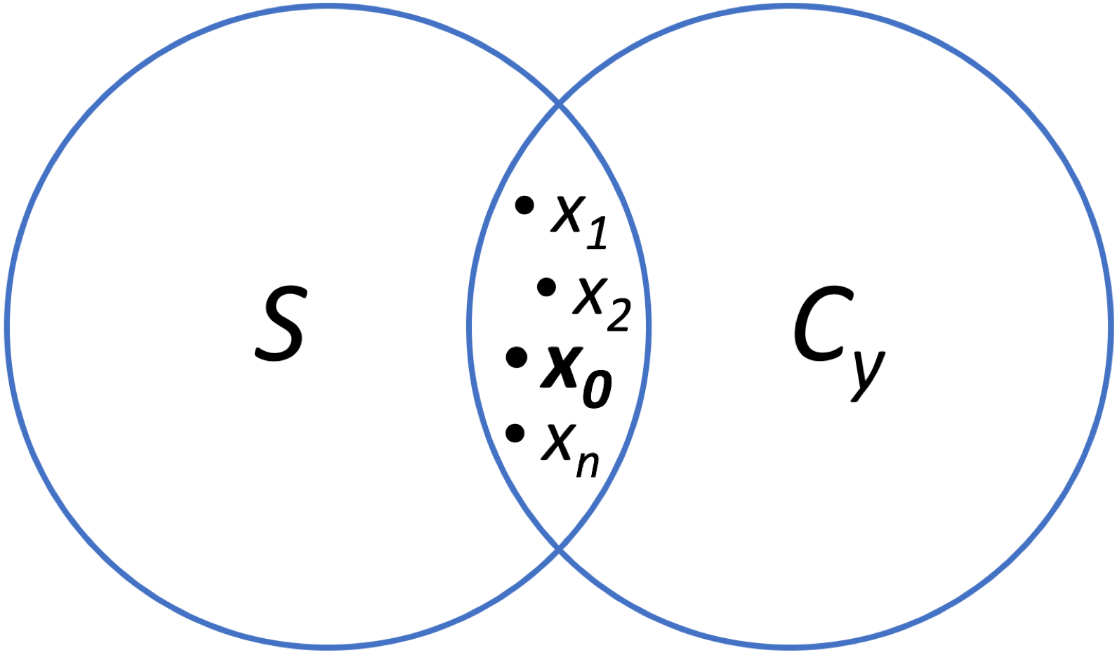
Problem Statement: More concretely, it stands to reason that there could exist multiple recovered images that look both realistic and feasible given a specific data acquisition process, and that one of these might represent hallucination. Thus, the objective of this work is to model the intersection between a clean image manifold $$$\mathcal{S}$$$ learned by a VAE-GAN and a data consistent subspace $$$\mathcal{C}_y := \{x \in \mathbb{C}^n: y = \Phi x\}$$$, since we could find hallucinated images $$$x_1$$$, $$$x_2$$$, or $$$x_n$$$, in addition to the true image $$$x_0$$$ (see Fig. 1).

Methods

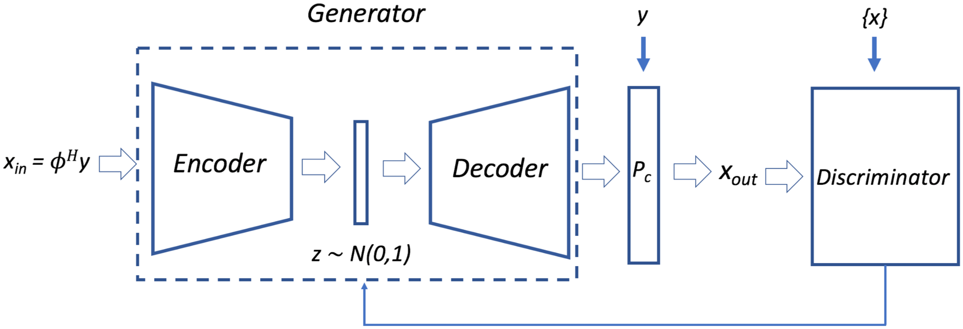
The VAE (which served as the generator function of the GAN) was composed of $$$4$$$ encoder layers and $$$4$$$ decoder layers. The encoder layers were formed through a sequence of strided convolution operations followed by ReLU activations and batch normalization. Latent space mean, $$$\mu$$$, and standard deviation, $$$\sigma$$$, were represented by fully connected layers. The decoder layers used transpose convolution operations for upsampling. At test time, latent code vectors were sampled from a normal distribution $$$z \sim \mathcal{N}(0,1)$$$ to generate new reconstructions that were evaluated for hallucinations. Data consistency was applied to all network outputs, which we found essential to obtaining high SNR. The discriminator function of the GAN was an 8-layer CNN. Figure 2 depicts the various components of the model.

The data consistent subspace was obtained by applying an affine projection based on the undersampling mask to ensure that reconstructions did not deviate from physical measurement.⁵ The VAE, in turn, was particularly useful to use as a generator function because it learns a probability distribution of realistic images that facilitates the exploration process of the manifold $$$\mathcal{S}$$$. By randomly sampling latent code vectors corresponding to specific images, then, we were able to traverse the space comprising $$$\mathcal{S}\cap\mathcal{C}_y$$$ to search for hallucinations.

Dataset. The knee dataset utilized in training and testing was obtained from $$$19$$$ patients with a 3T GE MR750 scanner.⁶ Each volume consisted of 320 2D slices of dimension $$$320\times256$$$, and a 5-fold variable density undersampling mask with radial view ordering was used to produce aliased input images $$$x_{\rm in}$$$ for the model to reconstruct.⁷

The loss functions used in training (shown below) were based on the L2 version of the GAN, where $$$\lambda$$$ is the GAN weight and $$$\eta$$$ controls the KL divergence weight).⁸

$$\min_{\Theta_d} \mathbb{E}_{x}\left[(1-\mathcal{D}(x;\Theta_d))^{2}\right] + \mathbb{E}_{y}\left[(\mathcal{D}(x_{\rm{out}};\Theta_d))^{2}\right]$$

$$\min_{\Theta_g} \mathbb{E}_{x,y} (1-\lambda)\left[\|x-x_{\rm{out}}\|_{2} + \eta D_{KL}(\mathcal{N}(\mu,\sigma)\|\mathcal{N}(0,1)) \right] + \lambda\mathbb{E}_{y}\left[(1 - \mathcal{D}(x_{\rm{out}};\Theta_d))^{2}\right]$$

Results

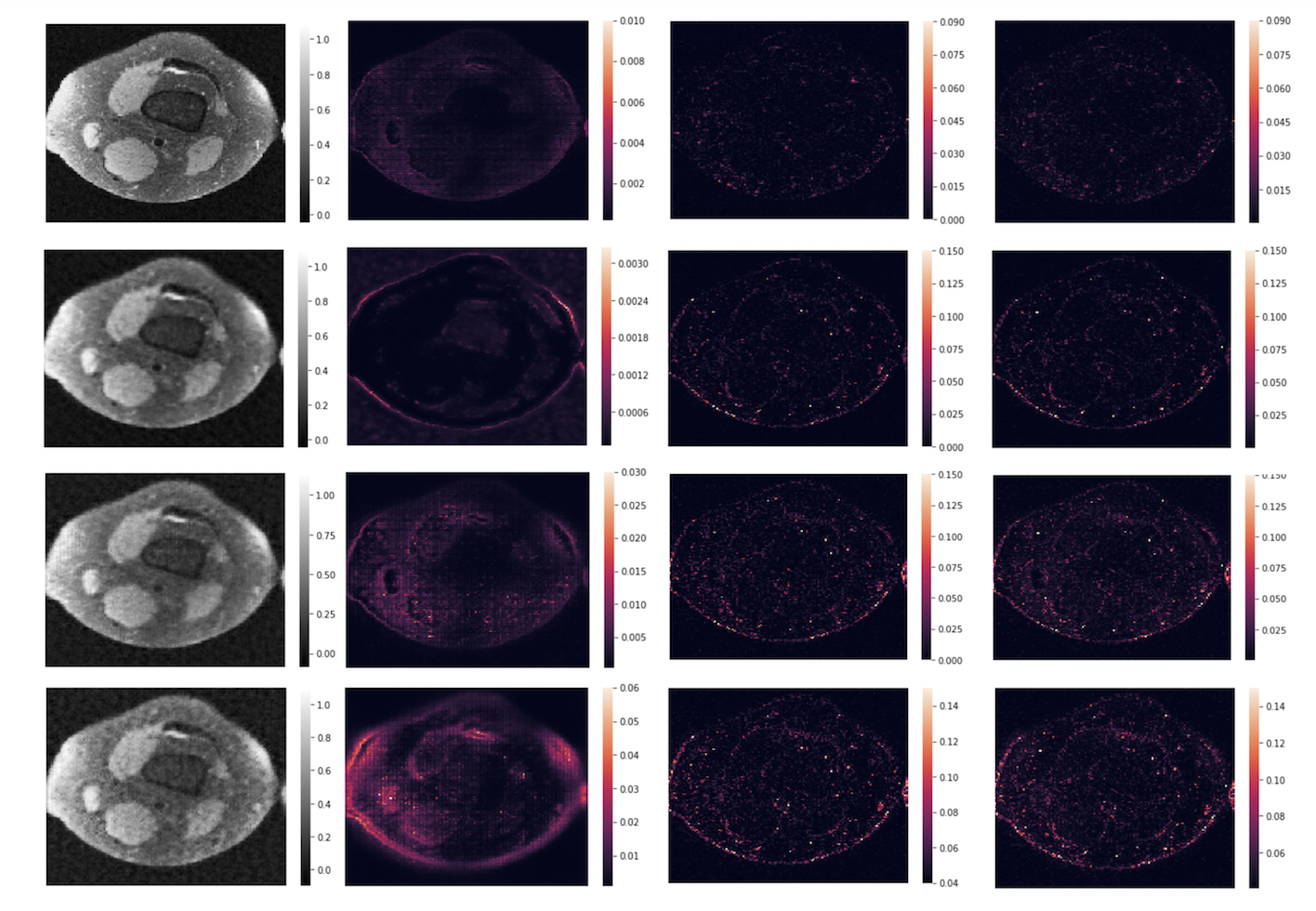
After training was completed, 1K outputs corresponding to different reference slices were generated by feeding a test image into the model and sampling from the resulting output distribution. To provide a better sense of the hallucination risks that can be attributed to the VAE-GAN architecture, we show the mean of the 1K reconstructed outputs for a representative slice and plot the pixel-wise variance, bias (using the mean image as the prediction), and error (Fig. 3), utilizing the common relation $$$error = bias^{2} + variance$$$.⁹ By showing both the difference from the mean and the inherent variability across realizations, in addition to inter-pixel dependencies, these plots provide information on the portions of a given image most susceptible to the introduction of realistic artifacts.

The results in Fig. 3 indicate that variance, bias, and error all increase as the undersampling rate increases (rows 1 and 3) and the GAN loss weight increases (rows 2 through 4). This indicates that high-frequency components of the image, which GANs are particularly adept at modeling and which highly undersampled images do not retain, pose the greatest risk in terms of hallucination. Nevertheless, with a reasonably conservative undersampling rate and choice of GAN weight $$$\lambda$$$, the probability of major hallucinations occurring is quite low.

Due to the influence of these parameters, ongoing work is focused on understanding the specific effects of different sampling trajectories on model robustness in addition to the development of regularization schemes capable of limiting hallucinations promoted by DL models in the high-frequency regime.

Acknowledgements

References

1. Tran Minh Quan, Thanh Nguyen-Duc, and Won-Ki Jeong. Compressed sensing MRI recon- struction with cyclic loss in generative adversarial networks. arXiv preprint arXiv:1709.00753, 2017.
   
2. Bo Zhu, Jeremiah Z Liu, Stephen F Cauley, Bruce R Rosen, and Matthew S Rosen. Image reconstruction by domain-transform manifold learning. Nature, 555(7697):487, 2018.
   
3. Li Xu, Jimmy SJ Ren, Ce Liu, and Jiaya Jia. Deep convolutional neural network for image deconvolution. In Advances in Neural Information Processing Systems, pages 1790–1798, 2014.
   
4. Guang Yang, Simiao Yu, Hao Dong, Greg Slabaugh, Pier Luigi Dragotti, Xujiong Ye, Fangde Liu, Simon Arridge, Jennifer Keegan, Yike Guo, et al. Dagan: Deep de-aliasing generative adversarial networks for fast compressed sensing MRI reconstruction. IEEE Transactions on Medical Imaging, 37(6):1310–1321, 2018.
   
5. Morteza Mardani, Enhao Gong, Joseph Y Cheng, Shreyas S Vasanawala, Greg Zaharchuk, Lei Xing, and John M Pauly. Deep generative adversarial neural networks for compressive sensing (GANCS) MRI. IEEE Transactions on Medical Imaging, 2018.
   
6. [online] http://mridata.org/fullysampled/knees.html.
   
7. Joseph Y Cheng, Tao Zhang, Marcus T Alley, Michael Lustig, Shreyas S Vasanawala, and John M Pauly. Variable-density radial view-ordering and sampling for time-optimized 3d cartesian imaging. In Proceedings of the ISMRM Workshop on Data Sampling and Image Reconstruction, 2013.
   
8. Alexey Dosovitskiy and Thomas Brox. Generating images with perceptual similarity metrics based on deep networks. In Advances in Neural Information Processing Systems, pages 658–666, 2016.
   
9. Robert Tibshirani. Bias, variance and prediction error for classification rules. Citeseer, 1996.