4762
A Generative Approach to Estimating Coil Sensitivities from Autocalibration data1Wellcome Centre for Human Neuroimaging, UCL Queen Square Institute of Neurology, University College London, London, United Kingdom
Synopsis
We present an algorithm for inferring sensitivities from low-resolution data, acquired either as an external calibration scan or as an autocalibration region integrated into an under-sampled acquisition. The sensitivity profiles of each coil, together with an unmodulated image common to all coils, are defined as penalised-maximum-likelihood parameters of a generative model of the calibration data. The model incorporates a smoothness constraint for the sensitivities and is efficiently inverted using Gauss-Newton optimization. Using both simulated and acquired data, we demonstrate that this approach can successfully estimate complex coil sensitivities over the full (FOV), and subsequently be used to unfold aliased images.
Introduction
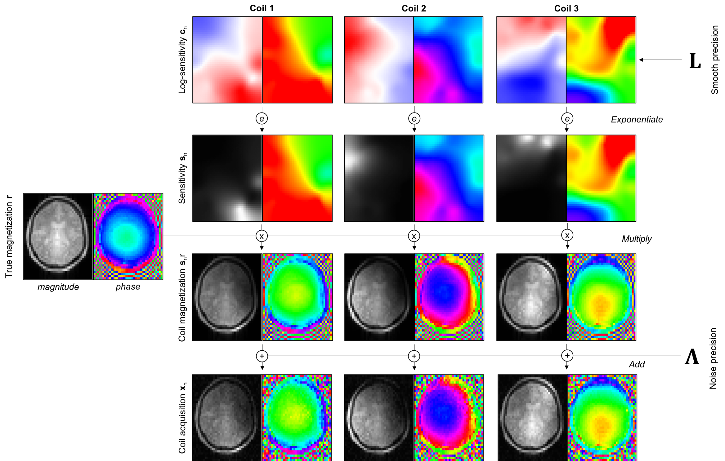
Parallel imaging relies on the spatial variance of the sensitivity of array-coil elements to unfold aliased images resulting from a sub-sampled acquisition. A variety of approaches to solving this problem exist1,2,3. SENSE-like methods require accurate estimation of each coil element’s sensitivity. These can be calculated by dividing the fully-sampled coil-wise images by some reference, e.g., a body-coil or the sum-of-squares across coil elements. However, these estimates are vulnerable to noise, particularly near signal voids and object boundaries, which introduce unrepresentative discontinuities. Smoothing can partly deal with noise but may exacerbate errors at discontinuities or signal voids. Here, we construct a generative model of the calibration data to address these problems (Figure 1). Sensitivities are inferred by optimizing the model likelihood. This approach can incorporate prior knowledge about the smoothness of the sensitivities and easily adapt to different noise levels. Furthermore, this approach provides an estimate of the complex sensitivity over the full field-of-view, thereby reducing sensitivity to motion, e.g. over the course of a time series in fMRI.Methods
Let us assume that each acquired image $$$\mathbf{x}_n\in\mathbb{C}^K$$$ is obtained from a true magnetization $$$\mathbf{r}\in\mathbb{C}^K$$$ multiplied by a sensitivity field $$$\mathbf{s}_n\in\mathbb{C}^K$$$ plus some Gaussian noise. Each sensitivity is assumed non-null and is therefore written as the exponential of another complex field: $$$\mathbf{s}_n=\exp\left(\mathbf{c}_n\right)$$$. The real part of $$$\mathbf{c}_n$$$ is the sensitivity’s log-magnitude ($$$\mathrm{Re}\left\{\mathbf{c}_n\right\}=\ln\left|\mathbf{s}_n\right|$$$); the imaginary part is the sensitivity’s phase ($$$\mathrm{Im}\left\{\mathbf{c}_n\right\}=\arg\left(\mathbf{s}_n\right)$$$). Smoothness is introduced by assuming that log-fields stem from a multivariate Gaussian with precision $$$\alpha_n\mathbf{L}$$$. This matrix is chosen to penalize sensitivities with high bending energy, under Neumann’s boundary conditions4. Finally, we incorporate noise correlation between coils with precision $$$\boldsymbol{\Lambda}$$$. Voxels are indexed by $$$k$$$, while coil-wise images and sensitivities at voxel $$$k$$$ are given by $$$\mathbf{x}_k\in\mathbb{C}^N$$$ and $$$\mathbf{s}_k\in\mathbb{C}^N$$$ respectively. The negative log-likelihood of the model is:
$$\mathcal{L}=\frac{1}{2}\sum_{k=1}^K\left(\mathbf{s}_kr_k-\mathbf{x}_k\right)^{H}\boldsymbol{\Lambda}\left(\mathbf{s}_kr_k-\mathbf{x}_k\right)+\frac{1}{2}\sum_{n=1}^N\alpha_n\mathbf{c}_n^{H}\mathbf{L}\mathbf{c}_n+\mathrm{constant}.$$
Differentiating with respect to the magnetization distribution yields a closed-form update:
$$r_k=\frac{\mathbf{b}_k^H\boldsymbol{\Lambda}\mathbf{x}_k}{\mathbf{b}_k^H\boldsymbol{\Lambda}\mathbf{b}_k}.$$
No closed-form solution exists for log-sensitivities, leading us to use a Gauss-Newton (GN) update scheme. The complex Hessian and gradient of the log-likelihood data term with respect to $$$\mathbf{c}_n$$$ have as many elements as voxels, with values:
$$g_{nk}=\frac{\partial\mathcal{L}}{{\partial}c_{nk}}=\frac{1}{2}\left({r_k}{r_k^\star}\right)s_{nk}\boldsymbol{\Lambda}_n\mathbf{s}_k^\star-\frac{1}{2}{r_k}{s_{nk}}\boldsymbol{\Lambda}_n\mathbf{x}_k^\star,$$
$$h_{nk}=\frac{\partial^2\mathcal{L}}{{\partial}c_{nk}^\star{\partial}c_{nk}}=\frac{1}{2}\Lambda_{nn}\left({r_k}{r_k^\star}\right)\left(s_{nk}s_{nk}^\star\right).$$
Gradient and Hessian with respect to the real and imaginary parts can be obtained from their complex equivalent5. We solve the GN inversion step, of the form $$$\left(\mathbf{H}+\alpha_n\mathbf{L}\right)^{-1}\left(\mathbf{g}+\alpha_n\mathbf{L}\mathbf{c}_n\right)$$$, by full-multigrid4. Since $$$\mathbf{r}$$$ is an exponentiated barycentre of $$$\mathbf{x}_{1{\dots}N}$$$, it can be shown that $$$\sum_n{\alpha_n}\mathbf{c}_n=\mathbf{0}$$$, which we enforce after each GN iteration.
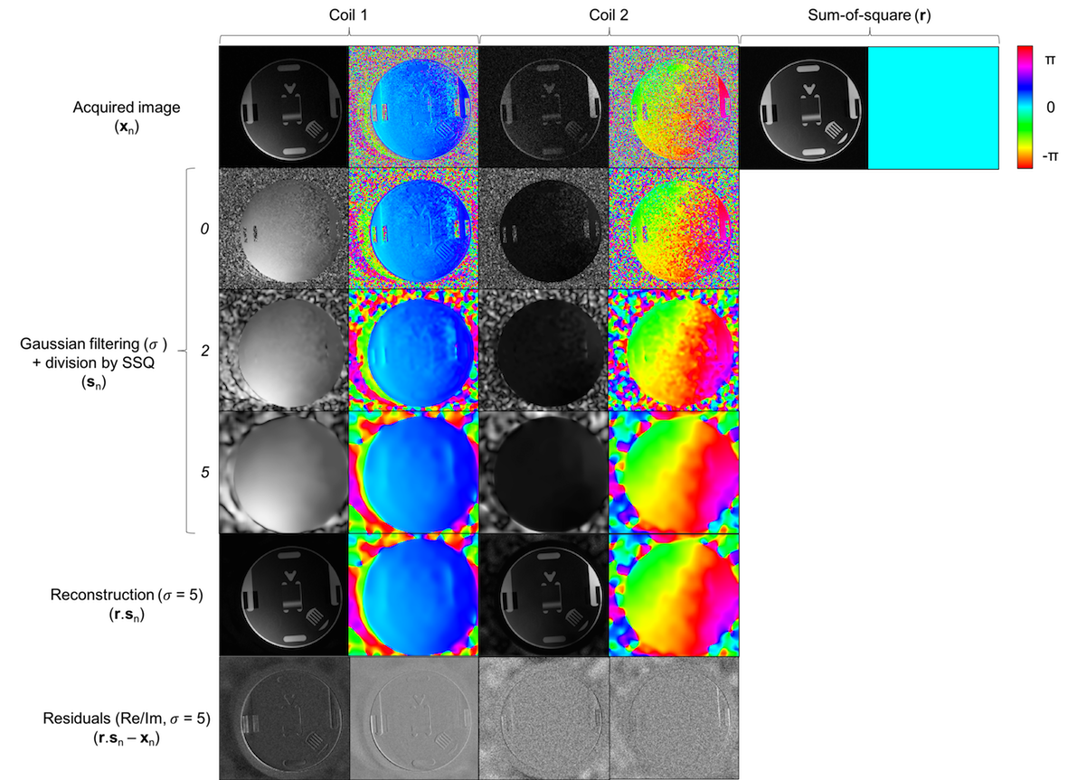
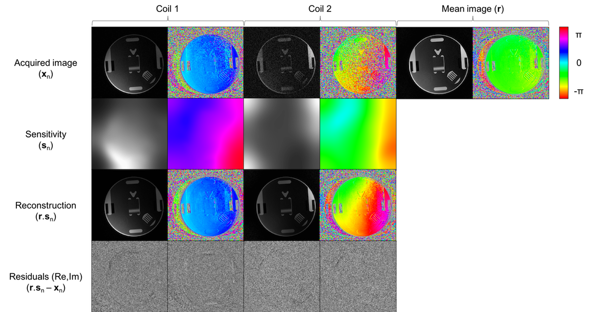
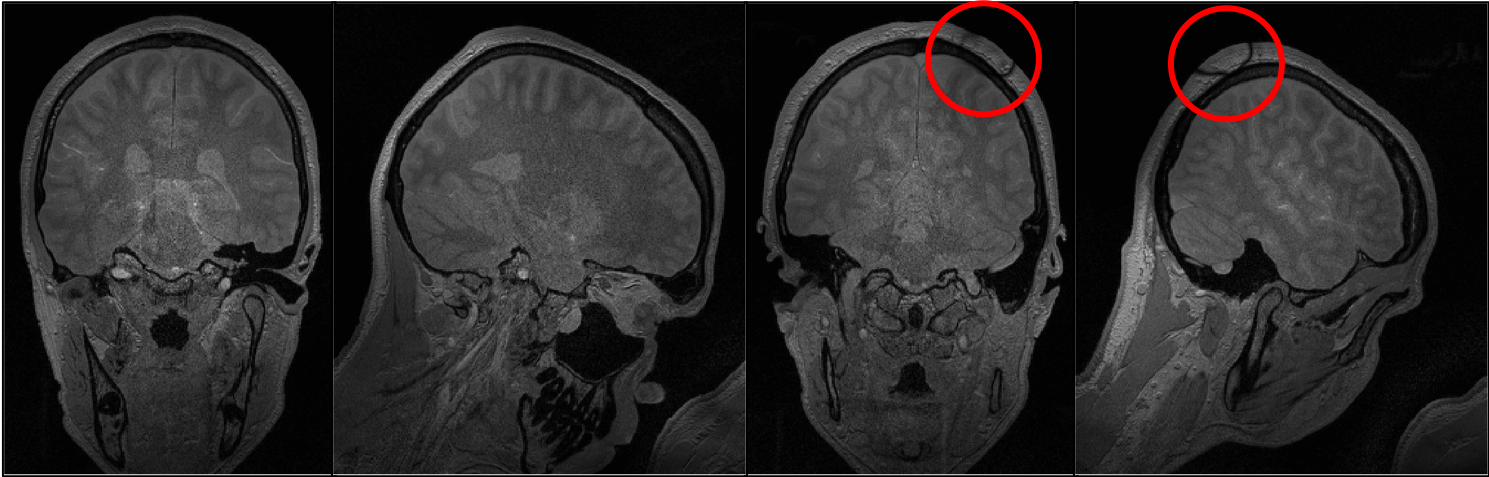
To validate our method, we applied it to a phantom image acquired with a 16-element-array-coil6. We compared our sensitivity estimates with fields obtained by smoothing the coil images and dividing them with their sum-of-squares. The noise covariance was assumed diagonal and its coil-specific elements were estimated by fitting a Rician mixture to each magnitude image.To evaluate the algorithm’s accuracy, we estimated sensitivity fields from the central autocalibration region of a 4-fold accelerated dataset acquired with a 64-element-array-coil. The sensitivities were then used to unfold the aliased images.
Results
The sensitivities estimated by normalising to the sum-of-squares show structured patterns, particularly in regions of low SNR, even with a large smoothing kernel, and are not estimated outside of the object resulting in high residuals (Figure 2). Conversely, sensitivities estimated with our proposed method are smooth, valid over the entire FoV, and in excellent agreement with the data, as evidenced by the residuals (Figure 3). When unfolding, our method yielded a good reconstruction without having to mask background voxels (Figure 4). However, some artefacts are present, which might be caused by near-zero sensitivities.Discussion
Most autocalibrated methods can be shown to provide or approximate maximum-likelihood solutions of the magnetization and sensitivity fields3 where smoothness is ensured by forbidding high spatial frequencies. In this work, we achieved this by using a prior distribution over (log)-sensitivities that incorporates prior belief about their smoothness. If a body-coil image is available, this can easily be incorporated into the model by treating it as an additional coil with $$$\alpha_{\mathrm{body}}\gg\alpha_{\mathrm{array}}$$$, reflecting our knowledge about its flatter sensitivity. We chose to penalise the log-sensitivity fields while, in reality, it is the real and imaginary parts that smoothly vary. However, this allows us to work in the exponentiated barycentre framework, which makes the optimization efficient by introducing an additional constraint on sensitivities.Conclusion
We have presented a generative framework for inferring sensitivities and mean magnetization from fully sampled acquisitions or arbitrary resolution. By doing so we can explicitly define and decouple various data generation phenomena and choose hyperparameters in a principled way. This model introduces prior belief to sensitivity estimation and could be extended to include partial sampling schemes and prior distributions over the mean magnetization, thereby unifying different common reconstruction algorithms.Acknowledgements
This work was supported by the MRC and Spinal Research Charity through the ERA-NET Neuron joint call (MR/R000050/1). The Wellcome Centre for Human Neuroimaging is supported by core funding from the Wellcome [203147/Z/16/Z]. The phantom dataset used in this study was acquired with support from the National Science Foundation through research grant CCF-1350563.References
- Pruessmann, K. P., Weiger, M., Scheidegger, M. B., & Boesiger, P. (1999). SENSE: sensitivity encoding for fast MRI. Magnetic resonance in medicine, 42(5), 952-962.ISO 690
- Griswold, M. A., Jakob, P. M., Heidemann, R. M., Nittka, M., Jellus, V., Wang, J., ... & Haase, A. (2002). Generalized autocalibrating partially parallel acquisitions (GRAPPA). Magnetic Resonance in Medicine: An Official Journal of the International Society for Magnetic Resonance in Medicine, 47(6), 1202-1210.ISO 690
- Uecker, M., Lai, P., Murphy, M. J., Virtue, P., Elad, M., Pauly, J. M., ... & Lustig, M. (2014). ESPIRiT—an eigenvalue approach to autocalibrating parallel MRI: where SENSE meets GRAPPA. Magnetic resonance in medicine, 71(3), 990-1001.
- Ashburner, J. (2007). A fast diffeomorphic image registration algorithm. Neuroimage, 38(1), 95-113.ISO 690
- Sorber, L., Barel, M. V., & Lathauwer, L. D. (2012). Unconstrained optimization of real functions in complex variables. SIAM Journal on Optimization, 22(3), 879-898.ISO 690
- Haldar, J. P.. Real MRI Dataset Samples. Retrieved from https://mr.usc.edu/download/data/.
Figures