4761
Accelerated Image Acquisition Using 2D Pulse Segments as Virtual Receivers for GRAPPA1School of Physics and Astronomy, University of Minnesota, Minneapolis, MN, United States, 2Center for Magnetic Resonance Research, Department of Radiology, University of Minnesota, Minneapolis, MN, United States, 3School of Mathematics, University of Minnesota, Minneapolis, MN, United States, 4Department of Electrical and Computer Engineering, University of Minnesota, Minneapolis, MN, United States
Synopsis
When based on a k-space description, 2D RF pulses can be applied in segments to increase the excitation bandwidth relative to a single-shot implementation, at a cost of increased imaging time. The increased imaging time can be overcome by undersampling the acquisition in one phase-encoded dimension, where data from each segment are viewed as originating from “virtual receive coils” rather than multiple physical coils. The undersampled data are reconstructed using parallel imaging techniques (e.g. as in GRAPPA). The method was tested in vivo with brain imaging, and the GRAPPA-like reconstruction was comparable in quality to a fully sampled reconstruction.
Purpose
Large magnetic field inhomogeneity (ΔB0) can be a significant cause of spatial flip-angle variation when using ordinary, limited-bandwidth RF pulses. Multidimensional RF pulses are particularly sensitive to inhomogeneity due to their extended pulse length, which decreases their bandwidth. Previously, it was shown that, by breaking a 2D pulse into multiple undersampled k-space segments, the excitation bandwidth can be increased at the expense of increased imaging time1,2,3. Here, we show how the redundant information from acquisitions of different pulse segments can be used to undersample acquisition k-space even when using a single receive coil. Data are recovered by treating each readout as originating from a virtual receiver in a GRAPPA-type4 reconstruction.Methods
Following previous work1, a 2D HS1 pulse was generated using 28 lines of k-space in the slow dimension (y). The time-bandwidth product (TBP) was set to 9 and the slab thickness to 5 cm in both dimensions of the pulse. Each subpulse element was 700 µs long. Two experiments were performed: 1) sampling the pulse in 4 segments, and 2) sampling it in 28 segments, the latter of which will hereafter be denoted “fully segmented.” The fully segmented pulse employed a rectangular autocalibrating signal (ACS) region to maximize the acceleration gained using this method. A larger dimension was chosen in the segmented (slow) direction of the 2D pulse which had the spatial encoding information (see. Fig. 2). A square region was used for the 4-segment pulse to increase the number of points available for the kernel weight calibration.
Experiments were performed with a Varian DirectDrive console (Agilent Technologies, Santa Clara, CA) interfaced to a 4T, 90-cm magnet (Oxford Magnet Technology, Oxfordshire, UK) with a clinical gradient system (model SC72, Siemens, Erlandgen, Germany). Experimental verifications of the fully segmented and 4-segment imaging sequences were performed using the same pulse parameters given above. The power for each segment in the 4-segment and the 28-segment pulse was set by comparing the RF amplitude (B1max ) determined from Bloch simulation to an experimental RF power calibration.
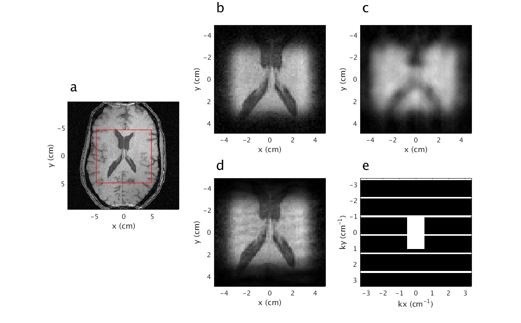
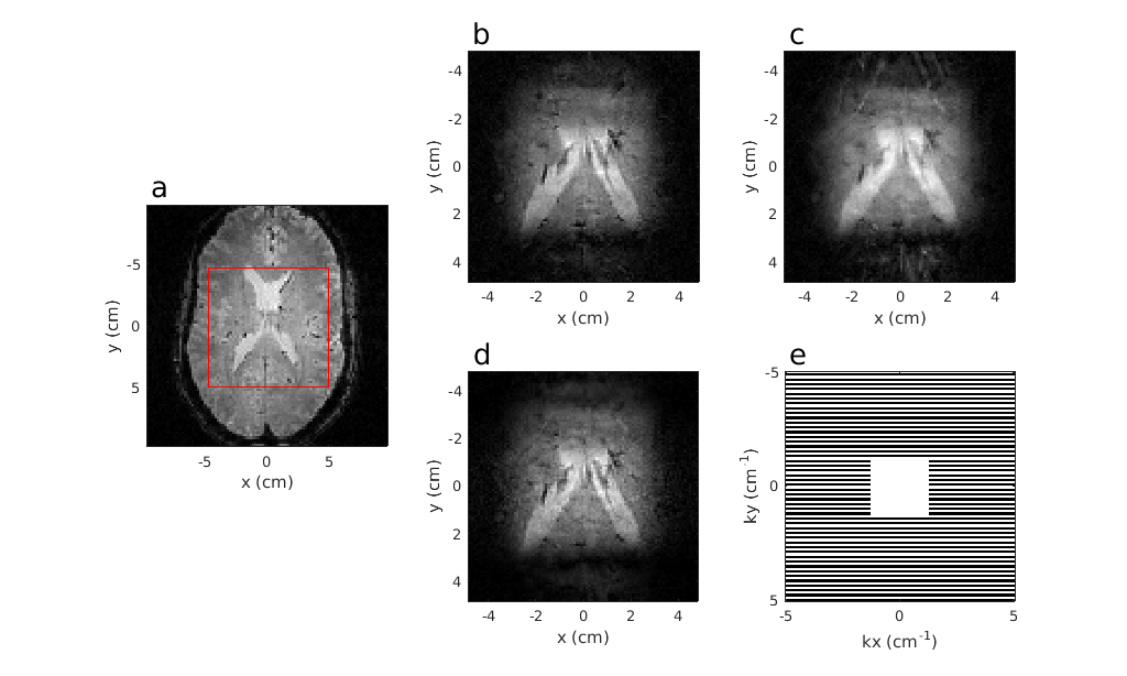
A 3D GRE sequence was used for both 28 and 4 segment excitations, with T1- and T*2-weighting, respectively. Sequence parameters are given in Figs. 3 and 4. The data for 2D excitation were fully sampled experimentally and downsampled retroactively for comparison. In both cases, the GRAPPA kernel was 3x2x3 in kx, ky, and kz, respectively. Every 11th line of ky was sampled on readout for the 28 segment pulse, with the central 10x20 lines of k-space fully sampled in the phase encoded dimensions, kx and ky, for use as ACS lines. For the 4-segment pulse, the central 32 lines were employed as ACS lines, while every 2nd line was sampled along ky on acquisition. In both cases, the ACS lines were used in the final reconstruction. The acceleration per pulse segment with these sampling patterns are R28 = 7.262 and R4 = 1.959.
Results
The real component of the Bloch-simulated transverse magnetization profiles for the 4-segment and fully segmented pulses are shown in Figs. 1 and 2, respectively. These clearly show the basis sets exploited to spatially encode signals with this method.
GRAPPA synthesized unsampled k-space data effectively when using the k-space data from the various pulse segments. The results for the fully segmented pulse are shown in Fig. 3, while those for the 4-segment pulse are displayed in Fig. 4. A slight discrepancy exists between the GRAPPA-reconstructed and fully sampled datasets.
Discussion
For the 4-segment excitation, with a fixed TR and resolution, the effective acceleration is Reff = 1.959. This is calculated as the product of the acceleration gained from data undersampling (R = 1.959) and from FOV reduction, divided by the number of pulse segments. The FOV reduction accelerates by a factor of 4 since the FOV was halved in both phase encoded dimensions relative to the reference acquisition. A similar calculation for the 28-segment pulse yields Reff = 1.037.
A discussion on employing traditional multiple receiver parallel imaging techniques4,5 in conjunction with this method is beyond the scope of the current work, but likely offers the possibility of higher acceleration factors than observed here when using a single receiver.
Conclusions
This work expands the utility of segmented 2D pulses as proposed by Mullen et al.1, Panych et al.2, and Hardy et al.3. The increased imaging time formerly associated with pulse segmentation has been overcome by taking advantage of the redundant information obtained between different pulse segments. Thus, segmented 2D pulses combined with data undersampling yield the increased excitation bandwidth of those pulses while simultaneously accelerating acquisition.
Acknowledgements
This work was supported by the National Institutes of Health grants U01 EB025153, P41 EB015894, and T32 EB008389.References
1. M. Mullen, N. Kobayashi, and M. Garwood, “2D Selective Excitation with Resilience to Large B0 Inhomogeneities.” Oral Presentation,” in Proceedings of the European Magnetic Resonance Meeting, 2018.
2. L. P. Panych and K. Oshio, “Selection of high-definition 2D virtual profiles with multiple RF pulse excitations along interleaved echo-planar k-space trajectories,” Magn. Reson. Med., vol. 41, no. 2, pp. 224–229, 1999.
3. C. J. Hardy and P. A. Bottomley, “31P Spectroscopic localization using pinwheel NMR excitation pulses,” Magn. Reson. Med., vol. 17, no. 2, pp. 315–327, 1991.
4. M. A. Griswold et al., “Generalized Autocalibrating Partially Parallel Acquisitions (GRAPPA),” Magn. Reson. Med., vol. 47, no. 6, pp. 1202–1210, 2002.
5. K. P. Pruessmann, M. Weiger, M. B. Scheidegger, and P. Boesiger, “SENSE sensitivity encoding for fast MRI,” Magn. Reson. Med., vol. 42, no. 5, pp. 952–962, 1999.
Figures
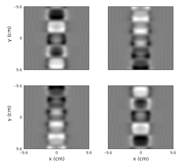
Figure 1: The real component of the transverse magnetization for each of the 2D pulse segments when traversed in 4 segments.
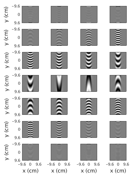
Figure 2: The real component of the transverse magnetization for each of the 2D pulse segments when fully segmented into 28 segments. The pulse parameters are described in the text.