4760
Simultaneous multislice reconstruction using spiral slice-GRAPPA1Biomedical Engineering, University of Virginia, Charlottesville, VA, United States, 2Medicine, University of Virginia, Charlottesville, VA, United States, 3Electrical and Computer Engineering, University of Virginia, Charlottesville, VA, United States, 4Radiology, University of Virginia, Charlottesville, VA, United States
Synopsis
Spiral trajectories provide efficient data acquisition and favorable motion properties for cardiac MRI. We developed multiband (MB) methods to accelerate spiral cardiac cine imaging including a non-iterative spiral slice-GRAPPA (SSG) reconstruction and a temporal SSG (TSSG). Using 25-35% of k-space for single-band calibration data, experiments in phantoms and five volunteers show 18.7% lower mean artifact power than CG-SENSE when imaging three slices simultaneously. TSSG incorporating CAIPIRINHA with temporal alternation and a temporal filter in reconstruction further reduced rRMSE by 11.2% compared to SSG.
Purpose
Spiral trajectories provide efficient data acquisition and favorable motion properties for cardiac MRI1. Multiband (MB) imaging with CAIPIRINHA3 has become an important acceleration method for Cartesian MRI2, 3, and it has also been demonstrated for non-Cartesian imaging4-6. For the non-Cartesian case, extensive calibration data are typically required, which extends the scan time4, 6. Cardiac MRI, which often involves dynamic imaging, also presents the opportunity to utilize temporal variation7, 8 to improve MB methods. We sought to develop improved MB methods for spiral cardiac MRI that require a reduced amount of calibration data and exploit temporal variation. We introduce spiral slice-GRAPPA (SSG) and temporal SSG (TSSG) and compare them to conjugate gradient sensitivity encoding (CG-SENSE) for MB spiral cine imaging.Theory
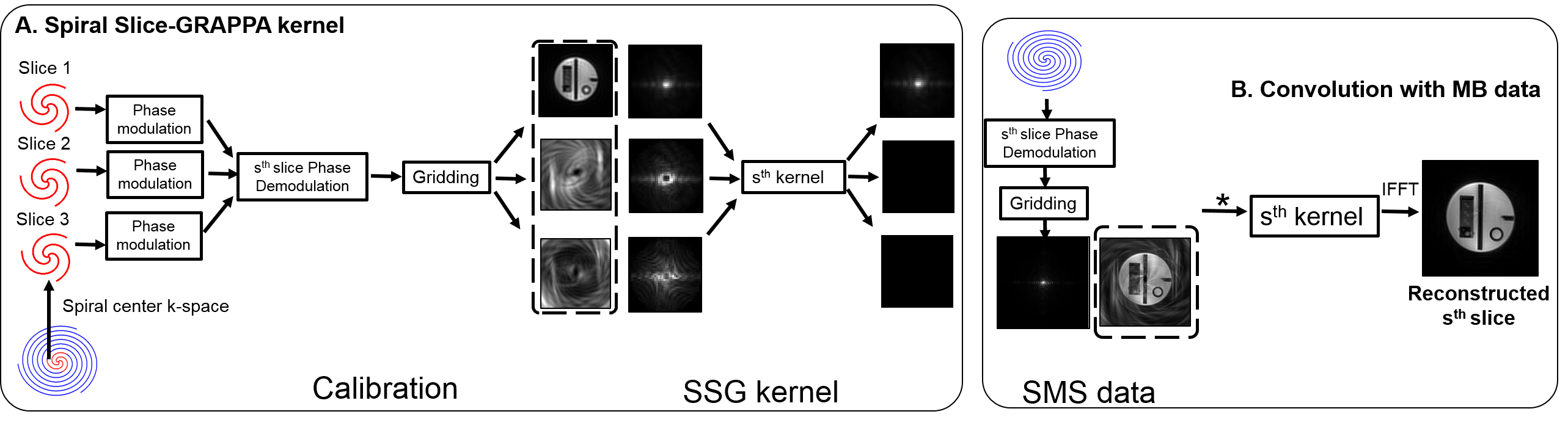
The SSG method is illustrated in Figure 1, and the SSG reconstruction model can be expressed as follows:
$$x_s=SSG_sC\left( P_{s}^{*}\cdot X \right),$$
where the matrix $$$SSG_s$$$ is the spiral slice-GRAPPA kernel of the $$$s^{th}$$$ slice, $$$C$$$ is the gridding function, $$$P$$$ represents CAIPIRINHA phase modulation, $$$X$$$ is the multiband k-space data, and $$$x_s$$$ is the separated k-space data of slice $$$s$$$. As shown in Fig. 1A, the $$$SSG_s$$$ kernel is fitted using the single-band (SB) spiral center of k-space as calibration data. For this calculation, CAIPIRINHA phase modulation is applied to all slices, then phase demodulation corresponding to the $$$s^{th}$$$ slice is applied to all slices. Next, gridding is performed on all slices, and the split-slice GRAPPA method2 is applied to fit the slice-GRAPPA kernel of the $$$s^{th}$$$ slice (Fig.1A). For image recovery, as shown in Figure 1B, the MB data are phase demodulated using the conjugate of the $$$s^{th}$$$ slice phase modulation matrix, $$$P_s^*$$$, and the gridding function $$$C$$$ is convolved with the MB data9. Next, the processed MB data are convolved with the $$$s^{th}$$$ slice-GRAPPA kernel, and the separated gridded k-space $$$(x_s)$$$ is obtained. Finally, the inverse Fast Fourier transform (IFFT) is performed to compute the image of the $$$s^{th}$$$ slice. This process is repeated for all slices. TSSG is based on alternation of CAIPIRINHA, and a temporal filter7, 8 is applied after SSG reconstruction.
Methods
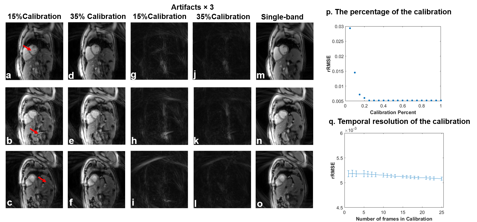
Spiral gradient-echo cine MRI was performed on a 3T system (Prisma, Siemens) using 30-34 RF channels. For MB cine RF excitation we employed CAIPIRINHA phase modulation of the multiple slices3, without and with temporal alternation of CAIPIRINHA phase. Simulations of MB images using SB data were performed in volunteers to determine the minimum amount of calibration data needed to minimize root mean squared error relative (rRMSE)10 to SB images. Also, for prospective MB spiral acquisitions, we compared the proposed SSG method with iterative CG-SENSE4. We also compared SSG to TSSG. Comparison studies used a phantom and short-axis cine MRI of five volunteers. SB images acquired at matched slice locations were used as reference standards. For MB imaging, SB kernel calibration data using the central 35% of k-space for each slice were acquired in one additional heartbeat appended to the cine acquisition.Results
Figure 2 shows that rRMSE is minimized when 25-35% of the SB k-space are used for kernel calibration. Example images reconstructed using 15% (a-c) and 35% (d-f) of k-space for calibration are shown, as are corresponding artifacts relative to fully-sampled SB reference images (g-l). Panels (p) and (q) show the dependence of rRMSE on the spatial and temporal resolution of the calibration data. Based on these results, subsequent MB acquisitions used 35% of k-space and one cardiac phase for the SB calibration data.
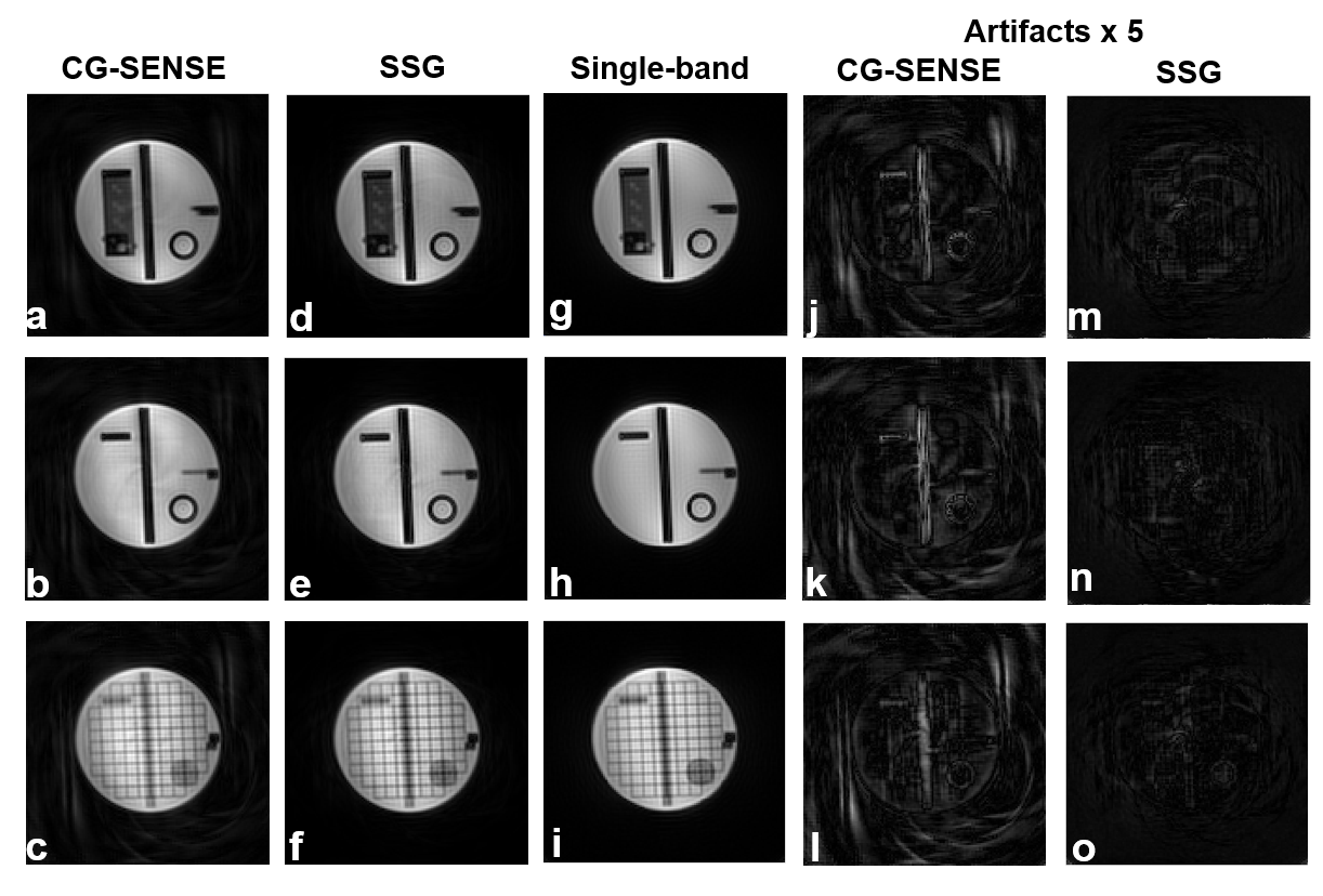
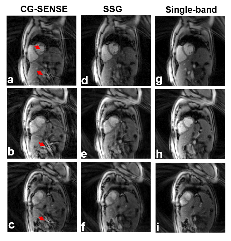
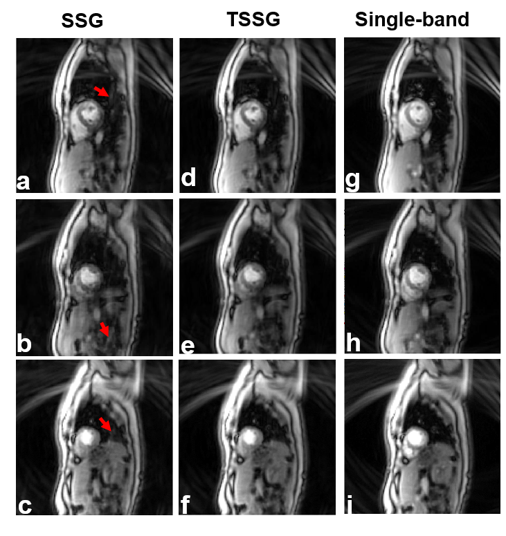
Figure 3 shows phantom results comparing SSG and CG-SENSE for MB=3, where both methods used 35% of SB k-space for calibration. Less slice leakage artifact was achieved using SSG. Results from a volunteer are shown in Figure 4. Specifically, for a reference, fully-sampled SB images at basal, mid-ventricular and apical locations are shown in Figure 4(g-i), and CG-SENSE-recovered MB images (a-c) and SSG-recovered MB images (d-f) at the same locations are also shown. Red arrows indicate slice-leakage artifacts in CG-SENSE, and these are reduced using SSG. The artifact power4 of SSG was 18.7% lower than CG-SENSE (0.148±0.036 vs 0.182±0.037 for SSG vs. CG-SENSE, p<0.05, N=5). SSG required 30% of the computation time of CG-SENSE. Figure 5 compares results using SSG (Fig.5 (a-c)) and TSSG (Fig.5 (d-f)). The mean rRMSE of TSSG was 11.2% lower than SSG. The computation time for TSSG is similar to SSG.
Discussion
SSG and TSSG are non-iterative slice-GRAPPA-based methods that provide better image quality than CG-SENSE for MB spiral cine MRI of the heart. Only 25-35% of the center of k-space is needed for kernel calibration, and the computation time is reduced. These methods provide rapid and accurate solutions for MB spiral imaging.Acknowledgements
Research support from Siemens Healthineers and the UVA Coulter Endowment.References
References: 1. Mayer et al. MRM, 1992, 28: 202-213. 2. Cauley et al. MRM, 2014, 72: 93 – 102. 3. Breuer et al. MRM, 2005; 53(3): 684-691. 4. Yutzy et al. MRM, 2011; 65(6): 1630-1637. 5.Yang et al. MRM, 2018, 00:1-11. 6. Chu et al. MRM, 2016; 76: 1196-1209. 7. Madore et al. MRM, 1999; 42: 813-828. 8. Kellman et al. MRM, 2001; 45(5): 846-852. 9. Fessler et al. IEEE T Signal Proces, 2003; 51(2): 560-574. 10. Chen et al. MRM, 2013; 72(4): 1028-1038.Figures