4735
Prostate and peripheral zone segmentation on multi-vendor MRIs using Deep Learning1Radiation Oncology, University of Miami, Miami, FL, United States
Synopsis
A Deep Learning algorithm for automatic segmentation of the prostate and its peripheral zone (PZ) is investigated across MR images from two MRI vendors. The proposed architecture is a 3D U-net that uses axial, coronal, and sagittal MRI series as input. When trained with Siemens MRI, the network achieves a Dice similarity coefficient (DSC) of .91 and .76 for the segmentation of the prostate and the PZ respectively. However, the network performs poorly on a GE dataset. Combining images from different MRI vendors is of paramount importance to pursue a universal algorithm for prostate and PZ segmentation.
INTRODUCTION
Accurate prostate segmentation is required for many clinical and research applications. Furthermore, due to the different imaging properties of the peripheral(PZ) and transition zones (TZ) of the prostate, accurate zonal segmentation is also necessary. The prostate and zonal contours are necessary for computer-aided diagnosis (CAD) applications for staging, diagnosis, and treatment planning for prostate cancer. Prostate MRI image segmentation has been an area of intense research. The advent of deep learning techniques, such as convolutional neural networks (CNN) has led to great success in image classification. 2, 3 Recently, the U-Net architecture has been proposed11 for medical imaging segmentation and has been applied to the prostate.4 In this work, we present a modification of the U-Net architecture for segmentation of both the prostate and PZ for creating a universal segmentation tool. The network is evaluated for images from two MRI vendors.METHODS
The prostate and PZ were manually contoured on T2-weighted axial MRI (T2W) in MIM (MIM Software Inc, Cleveland, OH, USA) by imaging experts. Two datasets were considered: (i) imaging data from the SPIE-AAPM-NCI PROSTATEx Challenge 13 (328 cases), acquired on two different types ofSiemens 3T MR scanners, and (ii) MRI data from patients in radiotherapy clinical trials at the University of Miami (100 cases), acquired on Discovery MR7503T MRI (GE, Waukesha, WI, USA).
The proposed preprocessing steps are: bias correction using the N4ITK algorithm,14 image normalization to an interval of [0,1], automatic selection of a region of interest (ROI), image re-sampling to a resolution of 0.5 × 0.5 × 0.5mm, and contour interpolation using optical flow.
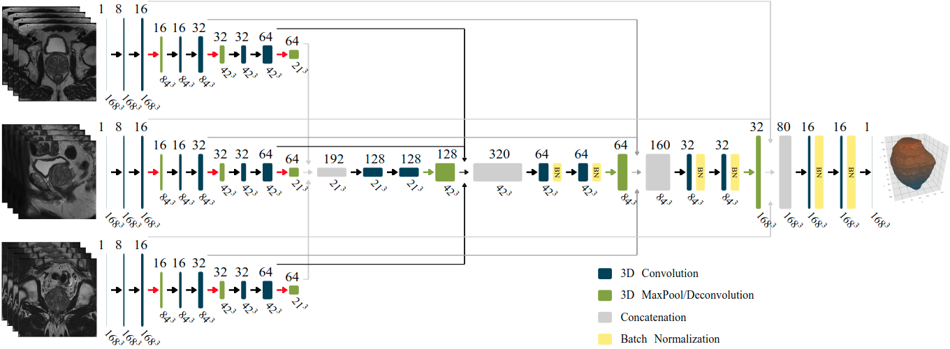
The proposed CNN consist of a 3D multistream architecture that follows the analysis and synthesis path of the 3D U-Net. 17 The input of each stream is the post-processed ROI for one of three MRI scans (axial, sagittal, and coronal), with a resolution of 1683. Figure 1 shows the proposed model, where all convolutional layers use a filter size of 3×3×3 and rectified linear unit (ReLu) as the activation function; with the exception of the last layer which uses a filter size of 1 × 1 × 1and Sigmoid as the activation function.
The dataset was split into 90% for training and 10% for validation. Also, in order to compare the robustness of the models with respect to changes in MRIvendor machines, a distinct model was trained for each dataset: GE (n=100), Siemens (n=328), combined model (n=428). A total number of 12 models were trained from the combination of three datasets, using or not data augmentation, and training for the segmentation of the prostate or the PZ.
RESULTS
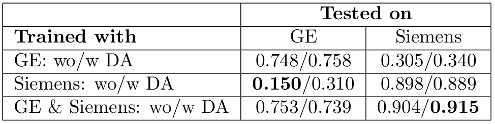
Table 1 shows the obtained DSCs for the segmentation of the prostate when the six trained models are used for the segmentation of the GE and Siemens dataset.
When the model is trained with the complete dataset and used to segment prostates from scans of a single MRI vendor the average DSCs are: 0.746 for GE and 0.909 for Siemens. In contrast, when the model is trained with examples from one MRI vendor and then used to process images from a different vendor the resulting DSCs are 0.322 and 0.257.
Table 2 shows the obtained DSCs for the segmentation of the PZ. The best DSCs (0.653 and 0.756) are obtained when the model is trained using the combined dataset.
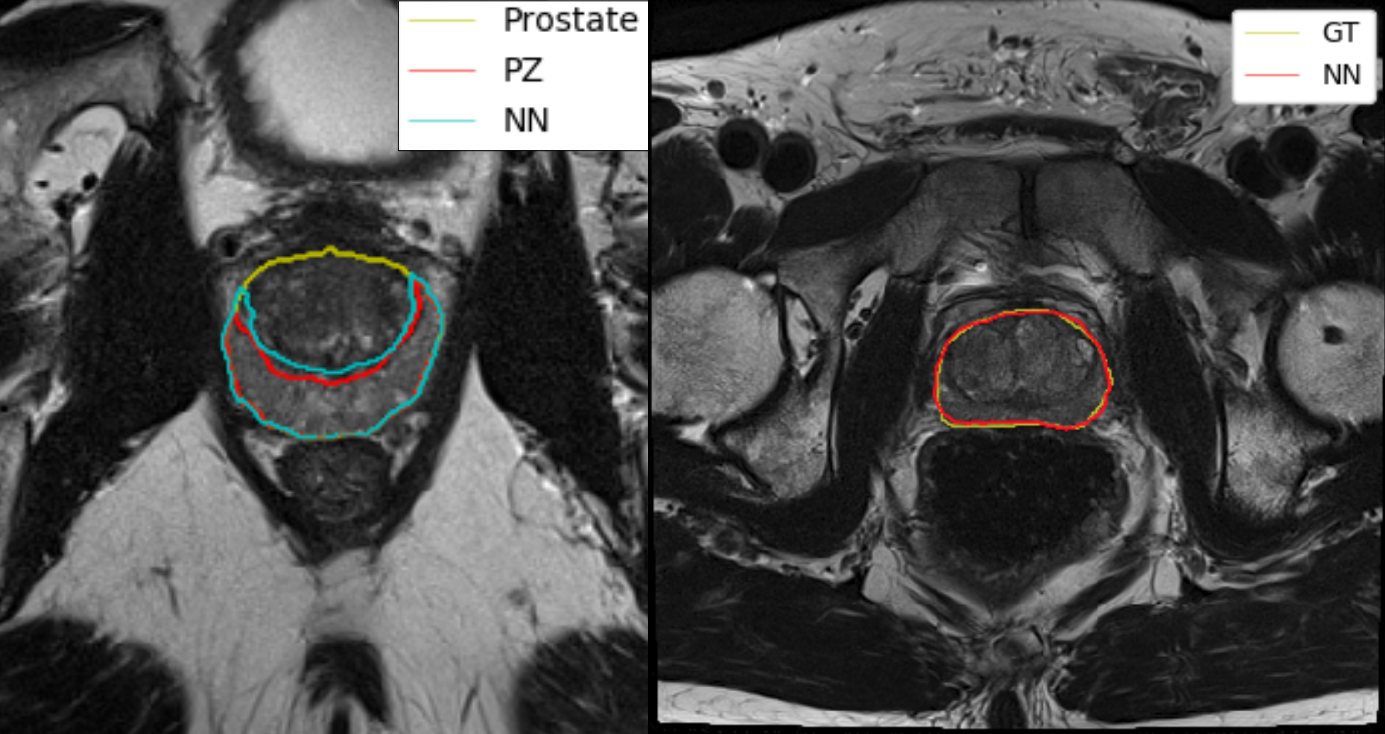
Figure 2 shows one example of prostate segmentation on the Siemens MRI vendor and a PZ segmentation on the GE MRI vendor. Both examples are from the middle layer of the prostate, and their corresponding DSCs are 0.906 and 0.742.
CONCLUSION
Our robustness tests show a strong sensibility of the proposed deep learning architecture with respect to the MRI vendor used in the training phase. This outcome implies that in order to build a universal deep learning algorithm, for prostate and peripheral zone segmentation, it will require joint efforts between institutions to build datasets with examples from all major MRI vendors.Acknowledgements
This work was supported by National Cancer Institute [R01CA189295 and R01CA190105]References
1. Litjens G, Toth R, van de Ven W, et al. Evaluation of prostate segmentation algorithms for MRI: The PROMISE12 challenge. Med Image Anal. 2014;18(2):359-373. doi:10.1016/j.media.2013.12.002
2. Krizhevsky A, Sutskever I, Hinton GE. ImageNet classification with deep convolutional neural networks. Commun ACM. 2017;60(6):84-90. doi:10.1145/3065386
3. Szegedy C, Wei Liu, Yangqing Jia, et al. Going deeper with convolutions. In: IEEE; 2015:1-9. doi:10.1109/CVPR.2015.7298594
4. Ronneberger O, Fischer P, Brox T. U-Net: Convolutional Networks for Biomedical Image Segmentation. In: Navab N, Hornegger J, Wells WM, Frangi AF, eds. Medical Image Computing and Computer-Assisted Intervention – MICCAI 2015. Vol 9351. Cham: Springer International Publishing; 2015:234-241. doi:10.1007/978-3-319-24574-4_28
5. Meyer A, Mehrtash A, Rak M, et al. Automatic high resolution segmentation of the prostate from multi-planar MRI. In: 2018 IEEE 15th International Symposium on Biomedical Imaging (ISBI 2018). Washington, DC: IEEE; 2018:177-181. doi:10.1109/ISBI.2018.8363549
6. Deukwoo K, Reis IM, Breto AL, et al. Classification of suspicious lesions on prostate multiparametric MRI using machine learning. J Med Imaging. 2018;5(03):034502. doi:10.1117/1.JMI.5.3.034502
7. Tustison NJ, Avants BB, Cook PA, et al. N4ITK: Improved N3 Bias Correction. IEEE Trans Med Imaging. 2010;29(6):1310-1320. doi:10.1109/TMI.2010.2046908
8. Farnebäck G. Two-Frame Motion Estimation Based on Polynomial Expansion. In: Bigun J, Gustavsson T, eds. Image Analysis. Vol 2749. Berlin, Heidelberg: Springer Berlin Heidelberg; 2003:363-370. doi:10.1007/3-540-45103-X_50
9. Çiçek Ö, Abdulkadir A, Lienkamp SS, Brox T, Ronneberger O. 3D U-Net: Learning Dense Volumetric Segmentation from Sparse Annotation. In: Ourselin S, Joskowicz L, Sabuncu MR, Unal G, Wells W, eds. Medical Image Computing and Computer-Assisted Intervention – MICCAI 2016. Vol 9901. Cham: Springer International Publishing; 2016:424-432. doi:10.1007/978-3-319-46723-8_49
Figures