4731
Beyond Dice Coefficient: Evaluating Shape Biomarker Preservation in Neural Network Segmentations1Radiology and Biomedical Imaging, University of California, San Francsico, San Francisco, CA, United States, 2Bioengineering, University of California, Berkeley, Berkeley, CA, United States, 3Center for Digital Health Innovation, University of California, San Francsico, San Francisco, CA, United States
Synopsis
High accuracy scores in volumetric overlap metrics, such as Dice Similarity Coefficient, have not been proven to be reliable indicators of shape biomarker preservation. This study proposes a novel approach towards quantitative evaluation of segmentations from neural networks using PCA and contrastive PCA.
Introduction
Osteoarthritis (OA) is one of the most common musculoskeletal conditions worldwide, with symptomatic hip OA significantly affecting the quality of life up to 4.2% of the population1. The pathophysiology of OA involves morphologic and biochemical changes in subchondral bone, articular cartilage, and synovial fluid, yet the precise etiology of the disease is unknown and treatment options are limited2. Previous research has demonstrated MR imaging biomarkers can stage and even predict the progression of OA (Knee OA: T1ρ/T2 3, bone shape4; Hip OA: T1ρ/T2 5,6, bone shape7). However, acquiring, segmenting, and analyzing images to extract biomarkers remains costly. Deep learning methods have shown high accuracy in segmentation tasks, but there is limited research on whether high accuracy is synonymous with biomarker preservation.
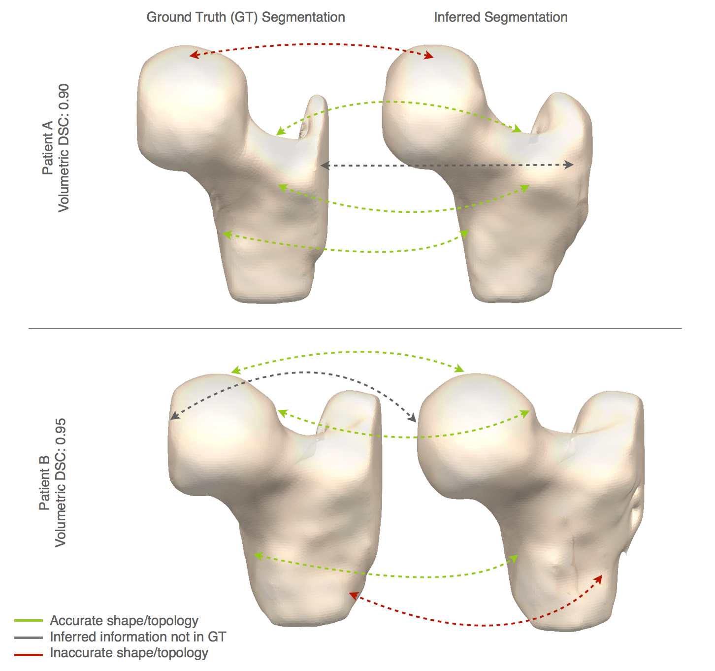
This study aims to establish a novel approach to compare deep-learning segmentation networks to assess shape biomarker preservation. These methods are applied on a hip MR dataset but are generalizable to any shape-related tasks. For example, Patient A and B in Figure 1 show areas of accurate and inaccurate shape/topology segmentation predicted by a neural network, yet both examples have high accuracy with volumetric Dice Similarity Coefficient (DSC)>0.90.
Methods
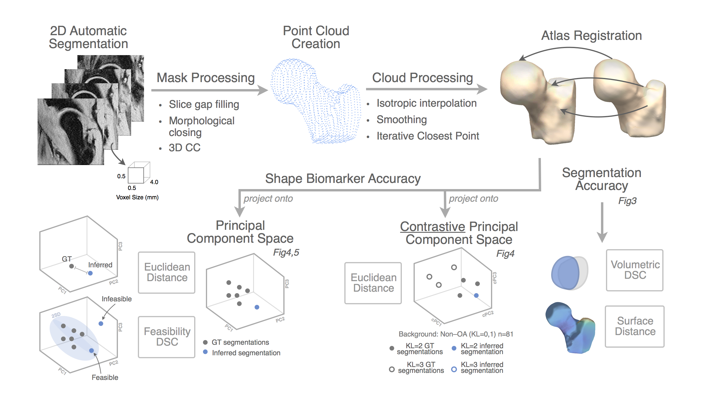
Figure2 provides an overview of the analysis methods. Inference is run on single slices and masks are stacked to create a volume. Volumetric DSC and surface distance are computed for baseline assessment of segmentation accuracy. Shape biomarker accuracy is assessed though shape modeling after mask processing. To address topological discontinuities, slice gaps are filled by interpolation of neighboring slices, morphological closing, and 3D connected component analysis. A point cloud is created from slice boundaries, interpolated to isotropic dimensions, aligned using ICP, and landmark matched with spectral correspondence. The registered points are projected onto existing shape spaces built by the ground truth segmentations.
The principal component (PC) and contrastive principal component (cPC)9. spaces are constructed only from the ground truth segmentations registered following the same process described above. This creates a compact space in which to meaningfully describe shape variation. Inferred images are projected into this space and shape biomarker accuracy is assessed via (1) the euclidean distance between each inferred shape and their ground truth in the shape space– perfect correspondence is 0 – and (2) the feasibility of resulting segmentations (within 2SD in each PC). Contrastive principal component analysis is a recently published technique to identify patterns in a dataset that are not present, or less present in a control dataset. OA GT segmentations were used to build the cPC space with non-OA GT segmentations as the background dataset. The contrastive principal component space describes the subtle shape variations within the OA population and can be used to identify subgroups. Only inferred shapes from patients with OA are projected into the cPC space and assessed via euclidean distance.
Results and Discussion
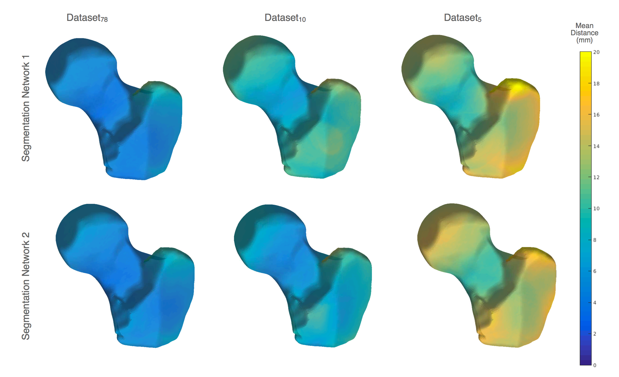
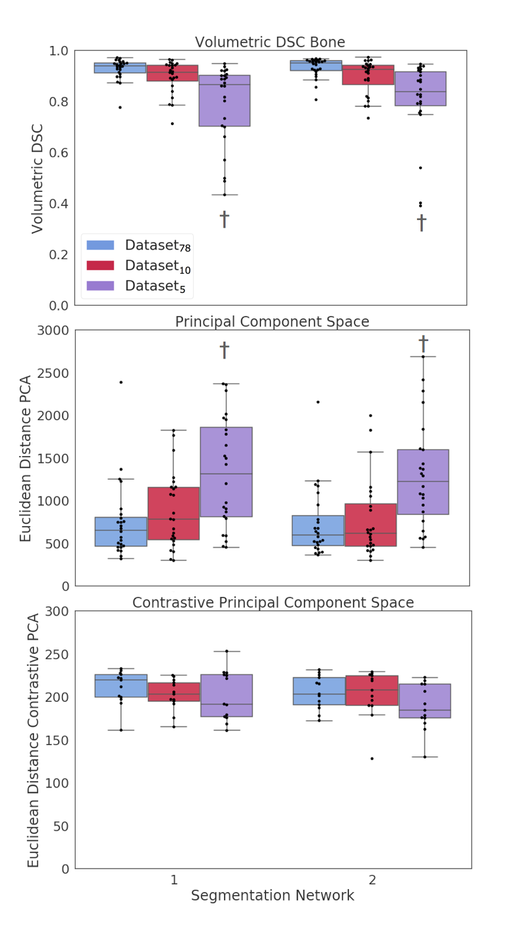
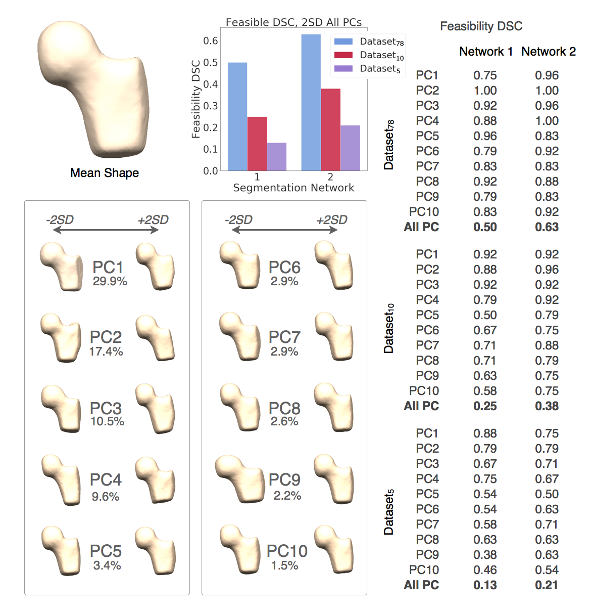
Network 1 and 2 show similar segmentation accuracies in mean distance, with Network 2 slightly outperforming Network 1 in Dataset10. Figure3 The greater trochanter the greatest errors, followed by the lateral shaft (possibly due to inconsistent GT segmentations on bookend slices). The femoral neck had the lowest segmentation error, and the femoral head was accurately segmented by both networks in Dataset10. Volumetric DSC performance was comparable between networks.Figure4 Dataset5 appeared to have ‘acceptable’ volumetric DSC (mean~0.85), but the segmentations did not preserve the shape features of interest as seen by the significant deviation from the GT in the PC space and the cPC space (OA space). Network 2 segmentations were marginally better at preserving the segmentations in the PC and cPC space. With Dataset78, 63% of segmentations by Network 2 fell within 2SD of all PCs, in comparison to 50% by Network 1. Figure5 Feasibility DSC sharply decreased for both networks with Dataset10 and Dataset5. Additionally, Network 2 had higher feasibility scores in the first principal components which explain the greatest amount of shape variability. These results suggest Network 2 is outperforming Network 1, but further investigation into the physical interpretation of each PC and their importance in the context of OA is warranted.Conclusion
High DSC scores were not indicative of preservation of shape biomarkers; low DSC scores however, were associated with loss of shape. If shape biomarkers extracted from deep learning segmentations are to be used for characterizing OA progression (or surgical planning, implant fitting, modeling, etc), it is necessary to look beyond Dice coefficient and evaluate networks on relevant shape features.
Acknowledgements
Funding sources: NIH ARP50AR060752, NIH AR R01046905, NIH K99AR070902References
1 Kim, Chan, et al. "Prevalence of radiographic and symptomatic hip osteoarthritis in an urban United States community: the Framingham osteoarthritis study." Arthritis & Rheumatology 66.11 (2014): 3013-3017.
2 Kapoor, Mohit, et al. "Role of proinflammatory cytokines in the pathophysiology of osteoarthritis." Nature Reviews Rheumatology 7.1 (2011): 33.
3 Prasad, A. P., et al. "T1ρ and T2 relaxation times predict progression of knee osteoarthritis." Osteoarthritis and cartilage 21.1 (2013): 69-76.
4 Neogi, Tuhina, et al. "Magnetic resonance imaging–based three‐dimensional bone shape of the knee predicts onset of knee osteoarthritis: data from the Osteoarthritis Initiative." Arthritis & Rheumatism 65.8 (2013): 2048-2058.
5 Gallo, Matthew C., et al. "T1ρ and T2 relaxation times are associated with progression of hip osteoarthritis." Osteoarthritis and cartilage 24.8 (2016): 1399-1407.
6 Pedoia, Valentina, et al. "Longitudinal study using voxel‐based relaxometry: Association between cartilage T1ρ and T2 and patient reported outcome changes in hip osteoarthritis." Journal of Magnetic Resonance Imaging 45.5 (2017): 1523-1533.
7 Pedoia, Valentina, et al. "Study of the interactions between proximal femur 3d bone shape, cartilage health, and biomechanics in patients with hip Osteoarthritis." Journal of Orthopaedic Research® 36.1 (2018): 330-341.
8 Ronneberger, Olaf, Philipp Fischer, and Thomas Brox. "U-net: Convolutional networks for biomedical image segmentation." International Conference on Medical image computing and computer-assisted intervention. Springer, Cham, 2015.
9 Abid, Abubakar, et al. "Exploring patterns enriched in a dataset with contrastive principal component analysis." Nature communications 9.1 (2018): 2134.
Figures