4711
Enforcing Structural Similarity in Deep Learning MR Image Reconstruction1Monash Biomedical Imaging, Monash University, Melbourne, Australia, 2School of Psychology, Monash University, Melbourne, Australia, 3Electrical and Computer System Engineering, Monash University, Melbourne, Australia, 4Institute of Medicine, Research Centre Juelich, Juelich, Australia
Synopsis
Deep Learning (DL) MR image reconstruction from undersampled data involves minimization of a loss function. The loss function to be minimized drives the DL training process and thus determine the features learned. Usually, a loss function such as mean squared error or mean absolute error is used as the similarity metric. Minimizing such loss function may not always predict visually pleasing images required by the radiologist. In order to predict visually appealing MR images in this work, we propose to use the difference of structural similarity as a regularizer along with the mean squared loss.
Introduction
Iterative reconstruction methods1 which enforce sparsity have been used for MR image reconstruction from undersampled data. The iterative methods are often used with regularizers to enforce a desired reconstructed image quality. For example, a total can be used to reconstruct smoother images or wavelet sparsity can be used for enhancing resolution at the expense of higher noise in the reconstructed images. Often a weighted linear combination of regularizers is used in order to achieve the desired image quality. Recently deep learning (DL) methods2,3,4 to perform such reconstructions have become an active area of research. The DL training process finds millions of network parameters that minimizes a cost function. Usually, the cost function to be minimized includes mean squared error or mean absolute error. In this work, we propose to use a difference of structural similarity as a regularizer together with the mean squared error to improve the quality of images reconstructed using a DL network.Methods
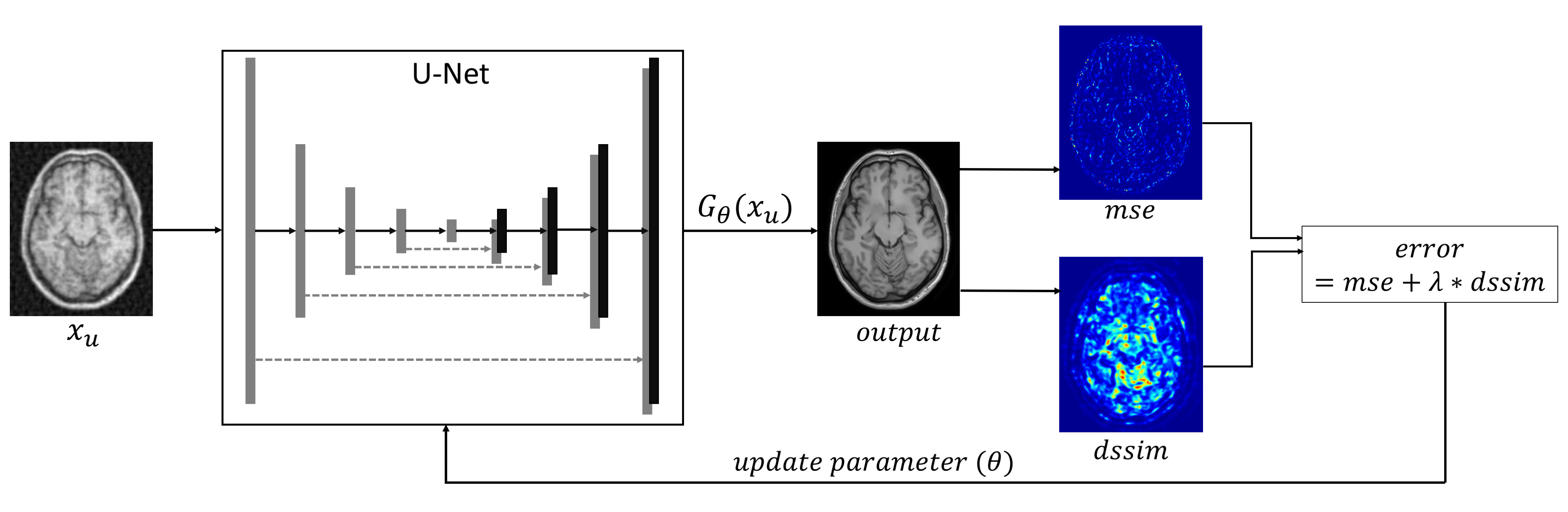
Network Architecture:
The network architecture and training process is illustrated in Figure 1. The network is a variation of the Unet5architecture with four maximum pooling stages and each stage consisting of three convolution layers. The number of channels were doubled after each maximum pooling layers and the first stage consisted of 64 channels.
Difference Structural Similarity Loss:
The structural similarity (SSIM)6 is a perceptual image quality metirc. The SSIM between a reference image ($$$x$$$) and an estimated image ($$$y$$$) is defined as:
$$SSIM(x, y) = \cfrac{(2\mu_{x'}\mu_{y'}+C1)(2\sigma_{x'}\sigma_{y'}+C2)}{(\mu_{x'}^2+\mu_{y'}^2+C1)(\sigma_{x'}^{2}+\sigma_{y'}^2+C2)}$$
where $$$\mu_{x'}$$$ is mean, $$$\sigma_{x'}$$$ is standard deviation for a small window of pixels in the image $$$x$$$. Similary, $$$\mu_{y'}$$$, $$$\sigma_{y'}$$$ are for the estimated image $$$y$$$; and $$$C1$$$ and $$$C2$$$ are constants determined by the dynamic range of the image. The $$$SSIM$$$ spans a range [0, 1], and in order to maximize in the DL reconstructed image, we define a difference structural similarity loss
$$dssim(x, y) = 1 - SSIM(x, y)$$
If $$$x_{ref}$$$ is a reference image and $$$x_{u}$$$ is an image with undersampling artefact then the reconstructed image from the DL network can be obtained as $$$\widehat{x} = G_\theta(x_u)$$$. A modified cost function to minimize is thus defined as
$$\min_{\theta} L(\theta) = || x_{ref} - G_\theta(x_u)||_{2}^2 + \lambda * dssim(x_{ref}, x_u) $$
We used T1 weighted images from the IXI database7, with 3D volumes from 254 subjects were used for training and 64 subjects were used for validation. The k-space data from the reference images were downsampled by a factor of 10 using 2D variable density undersampling to a generate training dataset which consisted of undersampling artefact. We trained two networks, one with simple mean squared error (Net-mse) and another with mean squared error along with $$$dssim (\lambda = 0.1)$$$ as a regularizer (Net-mse-dssim). The adam optimizer was used to train both the networks with a learning rate of 0.0001. The networks were trained for 100 epochs and the model for which validation loss was minimum was selected as the final trained network.
Results
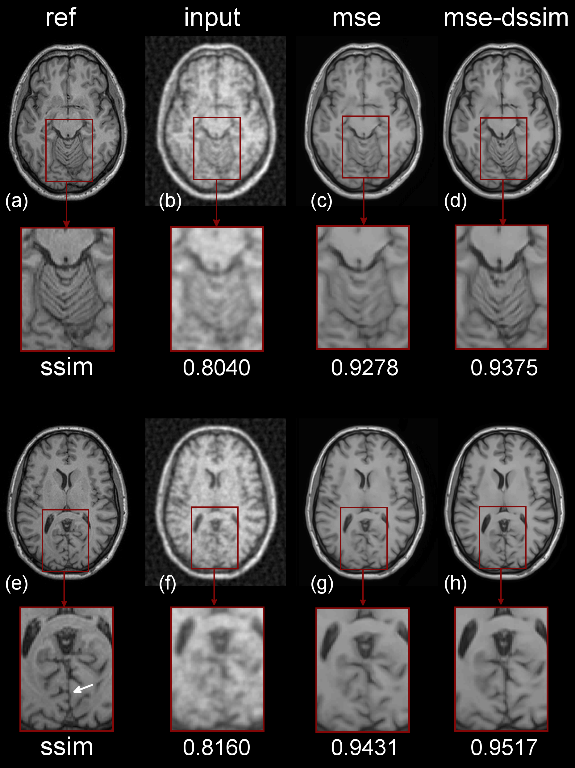
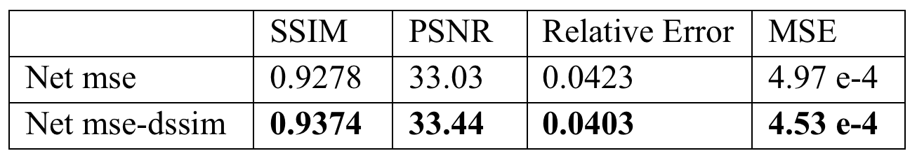
A representative result for the image reconstructions is shown in Figure 2 along with SSIM scores for two different slices on the validation dataset. For the network trained with the $$$dssim$$$ regularizer, the enlarged images in Figure 2 (c) show a better preservation of fine structural details. Similarly, sharp edges that were absent from Net-mse images are visible in the Net-mse-dssim images (edges near white arrow Figure 2 (e)). The Net-mse-dssim demonstrates improved quantitative scores based on several evaluation metrics (SSIM, PSNR, Relative Error, and MSE shown in Table 1).
Discussion
In this work, we have demonstrated that it is possible to enforce structural similarity during the convolutional neural network learning process, which yields images with high perceptual quality. This idea can be easily extended to include enhancement of other features with the use of appropriate regularizer loss function. For instance, an edge detection filter such as a Sobel filter could be applied to the DL output image and a difference-of-the-edges as a regularizer loss function could be used to enforce edge preservation.Conclusion
The $$$dssim$$$ regularizer when used with the mean squared loss function trains a DL model to provide T1 weighted MR images with high perceptual quality and an improved level of small anatomical detail. The framework presented is generic in nature and can easily be extended to include other regularizers.
Acknowledgements
No acknowledgement found.References
- Lustig M, Donoho D, Pauly JM. Sparse MRI: The application of compressed sensing for rapid MR imaging. Magnetic Resonance in Medicine: An Official Journal of the International Society for Magnetic Resonance in Medicine. 2007 Dec;58(6):1182-95.
- Zhu B, Liu JZ, Cauley SF, Rosen BR, Rosen MS. Image reconstruction by domain-transform manifold learning. Nature. 2018 Mar;555(7697):487.
- Wang S, Su Z, Ying L, Peng X, Zhu S, Liang F, Feng D, Liang D. Accelerating magnetic resonance imaging via deep learning. InBiomedical Imaging (ISBI), 2016 IEEE 13th International Symposium on 2016 Apr 13 (pp. 514-517). IEEE.
- Lee D, Yoo J, Ye J C. Compressed Sensing and Parallel MRI using Deep residual learning. ISMRM 2017; 0641
- Ronneberger O, Fischer P, Brox T. U-net: Convolutional networks for biomedical image segmentation. International Conference on Medical Image Computing and Computer-Assisted Intervention 2015 Oct 5 (pp. 234-241). Springer, Cham.
- Wang Z, Bovik AC, Sheikh HR, Simoncelli EP. Image quality assessment: from error visibility to structural similarity. IEEE transactions on image processing. 2004 Apr;13(4):600-12.
- https://brain-development.org/ixi-dataset/
Figures