4709
Accelerated MR image reconstruction using iterative feasible set projection1Seoul National University, Seoul, Korea, Republic of, 2AIRS medical, Seoul, Korea, Republic of, 3Department of Radiology, Seoul St. Mary’s Hospital, Seoul, Korea, Republic of, 4College of Medicine, The Catholic University of Korea, Seoul, Korea, Republic of
Synopsis
We proposed a new deep learning architecture for the reconstruction of highly undersampled data. The new architecture combines an iterative generative adversarial network (GAN) with a shared discriminator and interacts with data consistency blocks. The algorithm was applied to accelerate the data acquisition of the routine clinical protocols, particularly 2D Cartesian sampling sequences. The new method was tested to explore generalizability of the algorithm in in-vivo data under various conditions (difference pulse sequences, organs, coil types, sites, and health condition).
Purpose
The deep learning framework has been combined with parallel imaging or compressed sensing in order to utilize data-driven priors in addition to the multi-coil information and image priors1-3. Despite great potential of the deep learning for MR acquisition acceleration, end-to-end structural training may induce hallucinations that may not be explained by human intuition. To reduce unwanted hallucinations, we proposed an iterative feasible set projection method that enforces data consistency by gradient update after the feasible set projection by the generative adversarial network (GAN)4. The generalizability of the proposed method was tested using data from different pulse sequences, organs, coil types, sites, and health condition.Methods
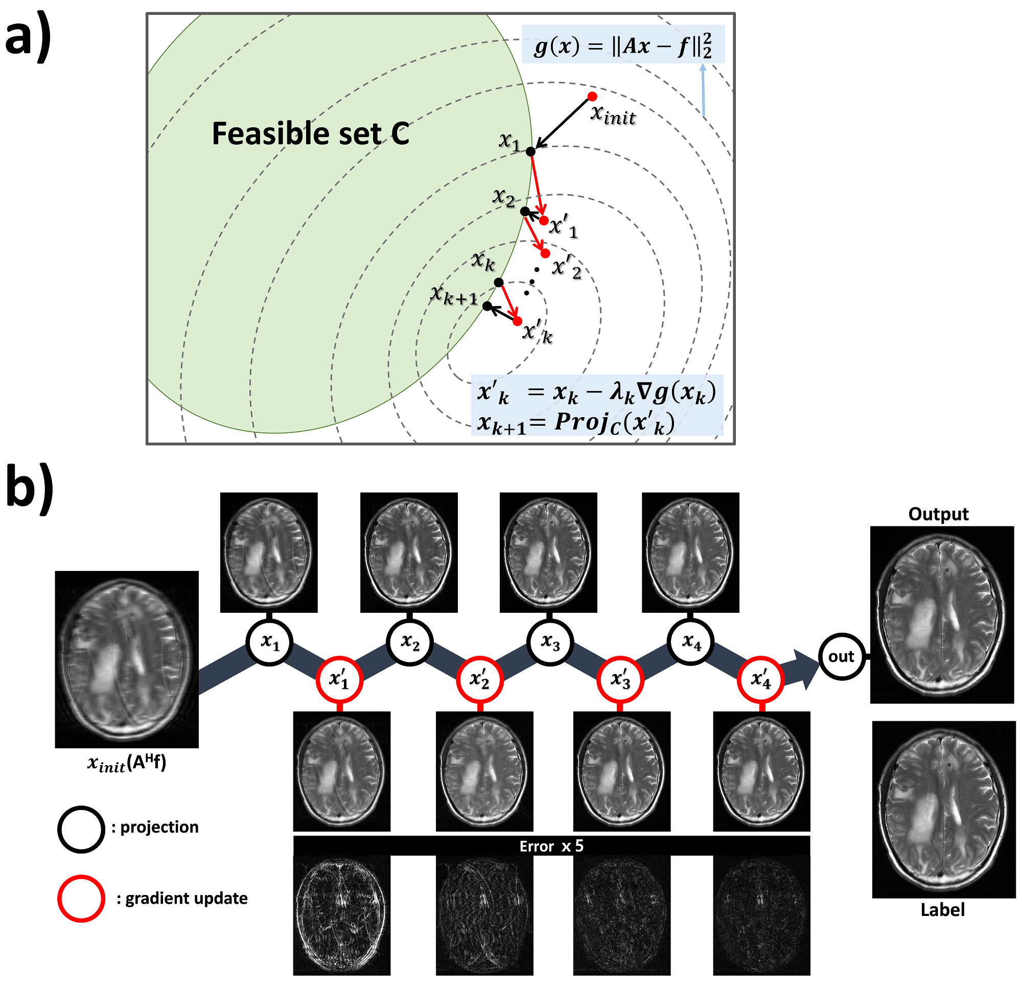
[Background & Algorithm] A feasible MR image manifold or subset C can be defined by sufficient data samples. When C is a closed convex set, a solution of the constrained problem, $$\underset{x\in C}{min}\frac{1}{2}\parallel{Ax-f}\parallel_{2}^2$$, can be iteratively solved by projected gradient descent5, $$x_{k+1}=Proj_c(x_{k}-\lambda_{k}A^HAx_{k}+\lambda_{k}A^{H}f)$$ , where $$$A$$$ includes Fourier transform, pixel-wise multiplication of coil sensitivities, and undersampling operator, $$$A^H$$$ is its adjoint operator, $$$\lambda_k$$$ is a step size and $$$f$$$ is measured data in the sensor domain (i.e. k-space). $$$Proj(·)$$$ is a projection operator, which can be performed by GAN that projects the input toward a feasible set C4,6. In detail, as depicted in Fig.1, each stage is comprised of a projection block using a generator network and a physics block, which updates solution using Landweber iteration7. The algorithm was implemented with 5 stages and a shared discriminator network. The loss function of the kth generator network $$$G_{\theta_{k,G}}$$$ in stage k is $$\underset{\theta_{1,G}\cdot\cdot\theta_{k,G}}{min}\frac{1}{N}\sum_{n=1}^{N}(G_{\theta_{k,G}}(x_{k,n}^{'})-x_{k,n}^{'})^2+(G_{\theta_{k,G}}(x_{k,n}^{'})-y_{n})^2+\gamma(D_{\theta_D}(G_{\theta_k,G}(x_{k,n}^{'}))-1)^2$$, where N is the total batch number, $$$x_k^{'}$$$ is an updated output of stage k (i.e.$$$x_{k}^{'}=x_{k}-\lambda_{k}A^HAx_{k}+\lambda_{k}A^Hf$$$), and $$$y$$$ is the label. $$$\gamma$$$ was set to 0.01. The first term of the loss function drives the generator network to minimize Euclidean distance between the input and the output of the networks, while the second term minimizes the difference between the label and the output of the networks. The third term represents an adversarial loss, which encourages the output to be driven to the manifold C. Note that the stage k includes training of the generator networks from $$$G_{\theta_{1,g}}$$$ to $$$G_{\theta_{k,g}}$$$. The discriminator network,$$$D_{\theta_D}$$$, classifies the feasible set element $$$y_n$$$ and the input $$$G_{\theta_{k,G}} (x_{k,n}^{'})$$$ . Therefore, the discriminator network is shared in all stages, and trained by the loss function: $$\underset{\theta_D}{min}\frac{1}{N}\sum_{n=1}^{N}(1-D_{\theta_{D}}(y_n))^2+D_{\theta_D}(G_{\theta_{k,G}}(x_{k,n}^{'}))^2$$.
[Training detail & procedure] Total 5 generator networks with the same structure of residual U-net8,9 were trained with different weights. The discriminator network consisted of 4-layers CNN and 2-fully connected layers (Fig. 1). The step size $$$\lambda_k$$$ was trained to the optimal values. The complex data was formed into 2 channels (real, imaginary) and fed into the network. The mini-batch size was 8, and Adam optimizer was used with learning rate 10-3 for 105 update iterations and 10-4 for another 105 update iterations.
[Data acquisition & process] Total 61 subjects were scanned with various pulse sequences, sites, number of channels, and target organs. The detailed information is listed on Fig.5a. Each pulse sequence was trained independently. All data were full-sampled and retrospectively undersampled (ACS line=32), then normalized by the norm of the k-space. Coil sensitivity maps were computed using ESPIRiT10.
Results
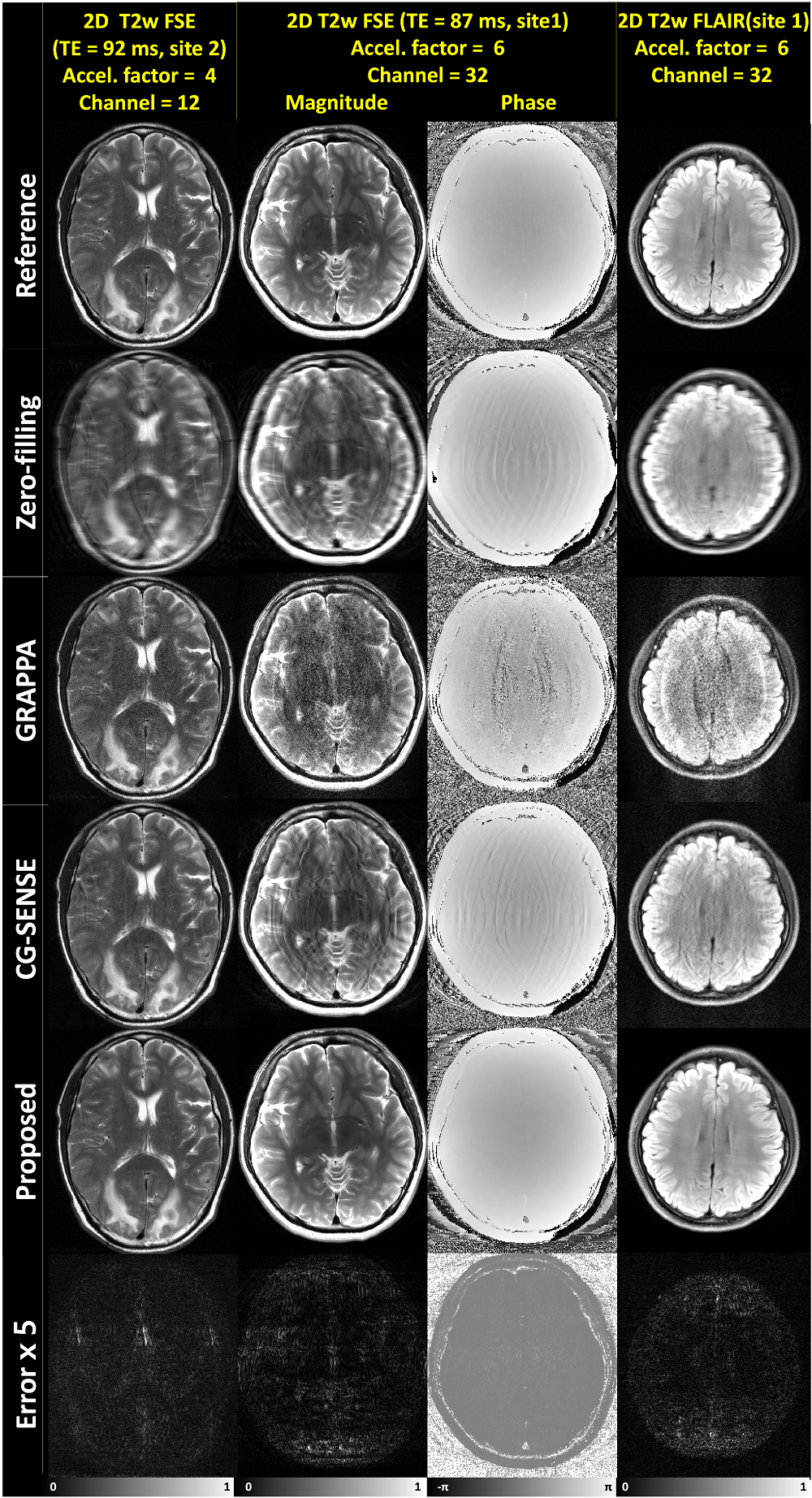
To interpret the characteristics of the algorithm, intermediate stage outputs of the representative test data from 2D T2w (neuro, site2) were depicted in Fig.2b. The absolute error maps between the label and the intermediate outputs indicated that the output converged to the probable solution as the stage progressed. Figure3 shows the reconstruction results of neuro data. For the regularly undersampled scheme, we compared our results with those processed with GRAPPA and CG-SENSE11,12. Our method successfully removed the aliasing artifacts even at the acceleration factor of 6. Other methods showed remaining artifacts. In particular, the patient with multiple metastasis (first column of Fig.3) demonstrates well-delineated lesions with no specific hallucination when compared to the reference. The network’s capability of handling complex data is demonstrated in column 2 and 3 of Fig.3. Figure4 shows the results of prostate data with zoomed images, demonstrating the algorithm can be applied to other organs as well. The superior results of the proposed algorithm were quantitatively supported by the quantity indices including PSNR, NRMSE, and SSIM13, which resulted in best values for all indices (Fig.5b).Conclusion and Discussion
In this work, we proposed a new deep learning architecture for an accelerated acquisition. The feasible-set projection method with enforced data consistency showed superior results compared to the conventional non-deep learning based methods. To further maximize the performance, the optimal number of stages and the network structure can be explored.Acknowledgements
This work was supported by Creative-Pioneering Researchers Program through SNU and Brain Korea 21 Plus Project in 2018.References
1. Hammernik K, Klatzer T, Kobler E, Recht MP, Sodickson DK, Pock T, Knoll F. Learning a variational network for reconstruction of accelerated MRI data. Magn Reson Med 2018;79(6):3055-3071.
2. Aggarwal HK, Mani MP, Jacob M. MoDL: Model Based Deep Learning Architecture for Inverse Problems. IEEE Transactions on Medical Imaging 2018.
3. Mardani M, Gong E, Cheng JY, Vasanawala SS, Zaharchuk G, Xing L, Pauly JM. Deep Generative Adversarial Neural Networks for Compressive Sensing (GANCS) MRI. IEEE Transactions on Medical Imaging 2018.
4. Goodfellow IJ, Pouget-Abadie J, Mirza M, Xu B, Warde-Farley D, Ozair S, Courville A, Bengio Y. Generative adversarial nets. 2014. p 2672-2680.
5. Eicke B. Iteration methods for convexly constrained ill-posed problems in Hilbert space. Numerical Functional Analysis and Optimization 1992;13(5-6):413-429.
6. Chang J-HR, Li C-L, Poczos B, Kumar BV, Sankaranarayanan AC. One Network to Solve Them All-Solving Linear Inverse Problems using Deep Projection Models. 2017. p 5889-5898.
7. Landweber L. An iteration formula for Fredholm integral equations of the first kind. American journal of mathematics 1951;73(3):615-624.
8. He K, Zhang X, Ren S, Sun J. Deep residual learning for image recognition. 2016. p 770-778.
9. Lee D, Yoo J, Ye JC. Deep residual learning for compressed sensing MRI. 2017. IEEE. p 15-18.
10. Uecker M, Lai P, Murphy MJ, Virtue P, Elad M, Pauly JM, Vasanawala SS, Lustig M. ESPIRiT—an eigenvalue approach to autocalibrating parallel MRI: where SENSE meets GRAPPA. Magn Reson Med 2014;71(3):990-1001.
11. Griswold MA, Jakob PM, Heidemann RM, Nittka M, Jellus V, Wang J, Kiefer B, Haase A. Generalized autocalibrating partially parallel acquisitions (GRAPPA). Magnetic Resonance in Medicine: An Official Journal of the International Society for Magnetic Resonance in Medicine 2002;47(6):1202-1210.
12. Pruessmann KP, Weiger M, Scheidegger MB, Boesiger P. SENSE: sensitivity encoding for fast MRI. Magn Reson Med 1999;42(5):952-962.
13. Wang Z, Bovik AC, Sheikh HR, Simoncelli EP. Image quality assessment: from error visibility to structural similarity. IEEE transactions on image processing 2004;13(4):600-612.
Figures