4702
Deep Partial Fourier Reconstruction1Electrical Engineering, Stanford University, Stanford, CA, United States, 2Radiology, Stanford University, Stanford, CA, United States, 3Bioengineering, Stanford University, Stanford, CA, United States
Synopsis
Standard methods for partial Fourier (PF) reconstruction do not perform well in the presence of significant phase variations. In this study, we propose a deep-learning-based approach for PF reconstruction (DPFR) to mitigate this issue. We compare DPFR results against standard methods (Homodyne, POCS) for in vivo images of the foot, leg, and abdomen. We demonstrate that DPFR achieves superior reconstruction quality, especially near phase boundaries, across a range of partial sampling parameters. Ultimately this may extend the applicability of partial Fourier reconstruction to instances where it is not commonly used.
Introduction
Partial Fourier (PF) sampling is routinely used in many fast imaging protocols, but standard PF reconstruction methods1,2 are known to perform poorly around significant phase variations3. Sources of such image phase variations range from system imperfections (e.g. susceptibility, B0) to deliberate encoding mechanisms (e.g. Dixon methods, phase contrast imaging). These phase variations pose a significant challenge for accelerating MRI.
Standard PF reconstruction methods1,2 are limited by two characteristics: (i) a priori phase estimation and (ii) single-dimensionality. The former artificially constrains the solution space and underutilizes high-frequency k-space, while the latter squanders spatial context. By framing PF reconstruction as a deconvolution problem (Figure 1), we identify a deep-learning-based approach that bypasses these limitations. We propose a deep convolutional neural network (CNN) for PF reconstruction and evaluate its performance in comparison with two standard methods: Homodyne1 and Projection Onto Convex Sets2 (POCS).
Methods
We employ a 10-layer CNN (Figure 2) to perform deep partial Fourier reconstruction (DPFR), mapping complex-valued zero-filled PF images back to fully sampled images. The general form of the CNN is motivated by recent work in deep-learning-based MRI reconstruction4,5,6. However unlike most deconvolution problems in imaging, the point spread function (PSF) for PF reconstruction is exactly known and reasonably compact (Figure 1). At partial Fourier fractions greater than 55%, over 80% of the PSF magnitude area lies within 10 pixels of center. With this in mind, we designed our CNN to operate on an appropriately sized pixel neighborhood.
Data from a variety of in vivo body MRI exams with significant phase variations were used to train, validate, and test the DPFR method. Our dataset comprised 53 patient exams of the foot, leg, and abdomen, acquired with IRB approval on 3T GE MR750 scanners using gradient-spoiled 3D dual-echo Dixon sequences. 38 patients were used for training, 5 for validation and 10 for testing. 1200 100x100 image slices were extracted from the individual Dixon echoes of each exam, for a total of 45600 training images.
We explored two key factors which scale the difficulty of the PF reconstruction task: the partial Fourier fraction (PFF) and the level of phase variations. We control the latter by multiplying the phase of the fully sampled image by $$$\alpha$$$ prior to retrospective partial Fourier sampling.
$$I=me^{i\alpha\phi}$$
Reconstruction performance was evaluated across a range of PFF (55%-80%) and $$$\alpha$$$ (0-2), using PSNR to evaluate similarity to the fully sampled image. Results were compared with the widely-used Homodyne, POCS, and the initial zero-filled reconstruction.
Results
Figures 3 and 4 provide a quantitative comparison of reconstruction quality for each method. DPFR outperformed all other methods for sufficiently large $$$\alpha$$$. This ordering was maintained across the entire range of partial sampling tested (PFF=55-80%).
Figure 5 illustrates the reconstruction of one representative test image. It is clear that POCS sharpens the image, but suffers from significant error near regions of rapidly varying phase such as water-fat boundaries. Homodyne outputs appeared similar but inferior. DPFR improves upon many of these localized errors.
Discussion
DPFR offers a promising alternative to POCS and Homodyne when sharp variations in phase are present. It demonstrated robustness across a range of phase multipliers, PFFs, and anatomy. The latter is especially important as it demonstrates the generalizability, and thus practicality, of DPFR.
POCS and Homodyne should not be expected to perform well on our dataset under normal conditions ($$$\alpha$$$ = 1) because large phase variations were naturally present. The purpose of this work was to demonstrate the limited range of applicability of POCS/Homodyne and to propose an alternative approach for images outside this regime. With this in mind, DPFR is most suitable for gradient echo sequences and phase-based imaging sequences such as phase contrast and Dixon.
The inverse problem of recovering a fully-sampled complex-valued image from partially acquired k-space is ill-posed. What sets DPFR apart from POCS/Homodyne is that it has the capacity to incorporate additional prior information while also eliminating unrealistic phase constraints. The solution space is no longer constrained by an initial phase estimate, and the network has the capacity to glean context from two spatial dimensions rather than one. Moreover, DPFR can be tuned to the specific phase characteristics and PSF of a given sequence and PFF.
Conclusion
DPFR can improve robustness to phase variations when reconstructing partial Fourier images. This is relevant to MR sequences where phase variations are significant and fast imaging is desired, including Dixon sequences, phase contrast imaging, and gradient echo sequences. Future research should focus on integrating DPFR with complementary acceleration methods like parallel imaging and compressed sensing.Acknowledgements
Research support provided by R01 EB009690, R01 EB026136, and GE Healthcare.References
1. Noll DC, Nishimura DG, Macovski A. Homodyne detection in magnetic resonance imaging. IEEE Trans Med Imaging. 1991;10(2):154-163.
2. Haacke E., Lindskogj E., Lin W. A fast, iterative, partial-fourier technique capable of local phase recovery. J Magn Reson.1991;92(1):126-145.
3. McGibney G, Smith MR, Nichols ST, Crawley A. Quantitative evaluation of several partial Fourier reconstruction algorithms used in MRI. Magn Reson Med. 1993;30(1):51-59.
4. Schlemper J, Caballero J, Hajnal JV, Price A, Rueckert D. A Deep Cascade of Convolutional Neural Networks for MR Image Reconstruction. In: Niethammer M, Styner M, Aylward S, et al., eds. Inf Process Med Imaging. Vol 10265. Cham: Springer International Publishing; 2017:647-658.
5. Cheng JY, Chen F, Alley MT, Pauly JM, Vasanawala SS. Highly Scalable Image Reconstruction using Deep Neural Networks with Bandpass Filtering. arXiv:180503300 [physics]. May 2018. http://arxiv.org/abs/1805.03300. Accessed July 16, 2018.
6. Wang S, Su Z, Ying L, et al. Accelerating magnetic resonance imaging via deep learning. Proc IEEE Int Symp Biomed Imaging. 2016:514-517.
7. Kingma DP, Ba J. Adam: A Method for Stochastic Optimization. arXiv:14126980 [cs]. December 2014. http://arxiv.org/abs/1412.6980. Accessed November 7, 2018.
Figures
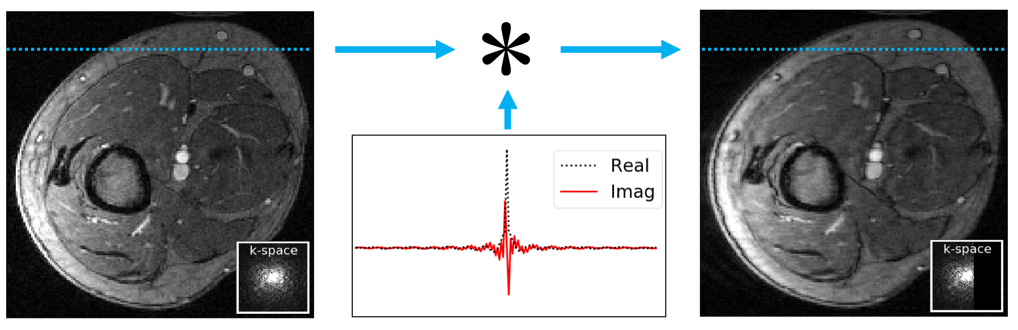
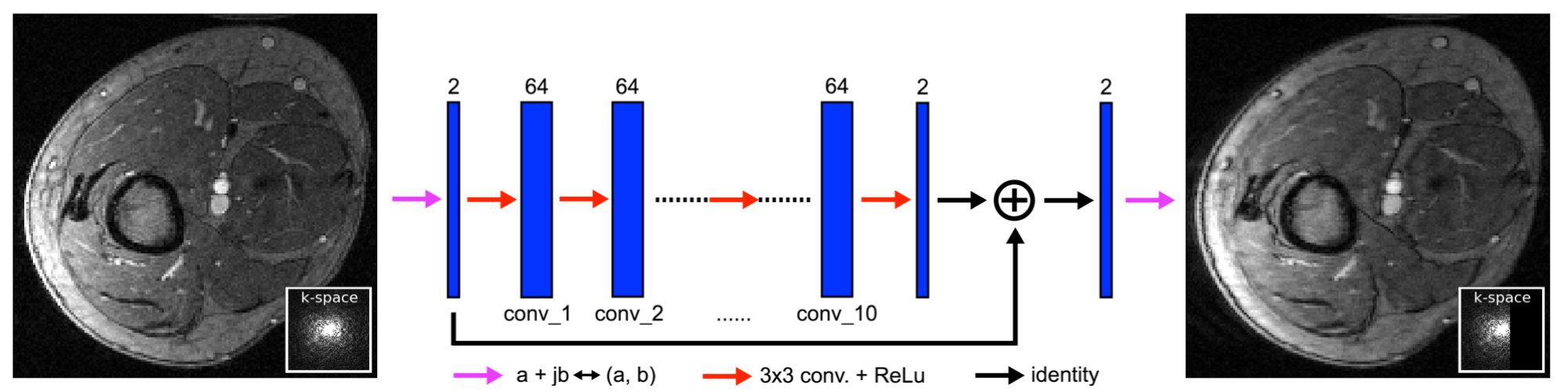
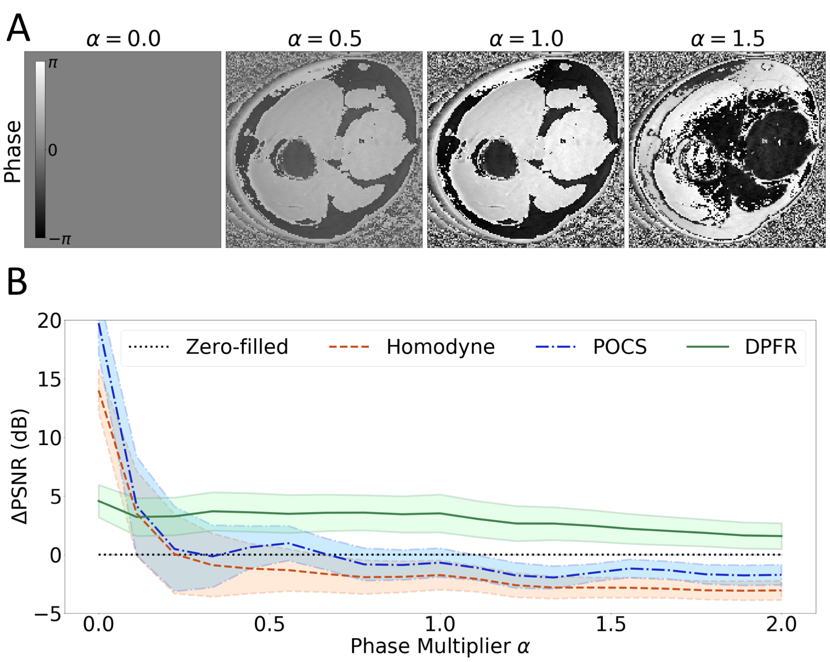
Figure 3. A: Phase of a fully sampled image after retrospective phase scaling with parameter α. We adjust α to study reconstruction robustness to phase variations. α = 1 represents the true phase of the image. B: Comparison of partial Fourier reconstruction methods across a range of phase scaling. ΔPSNR is the difference between the PSNR of the reconstructed output and the zero-filled input. Results are calculated on 6000 complex-valued images from 10 in vivo exams not seen during training. Bold lines and shaded areas represent the mean and standard deviation of ΔPSNR respectively.
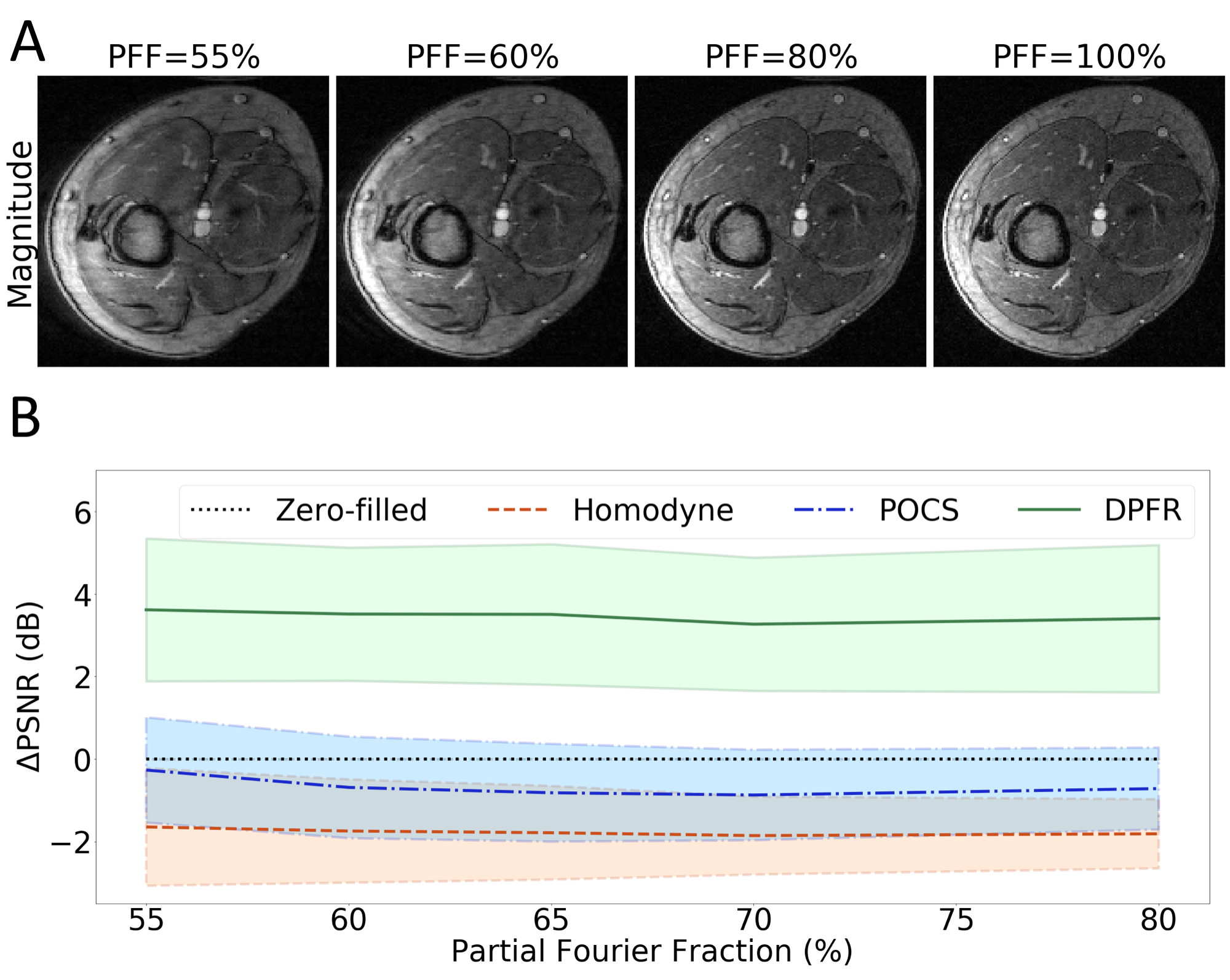
Figure 4. A: Magnitude of a zero-filled partial Fourier image at various partial Fourier fractions (PFF), with α = 1 (no phase scaling). Decreasing the PFF increases horizontal blurring. PFF=100% represents the fully sampled case. B: Comparison of partial Fourier reconstruction methods across a range of PFFs, with α = 1 (no phase scaling). ΔPSNR is the difference between the PSNR of the reconstructed output and the zero-filled input. Results are calculated on 6000 complex-valued images from 10 in vivo exams not seen during training. Bold lines and shaded areas represent the mean and standard deviation of ΔPSNR respectively.
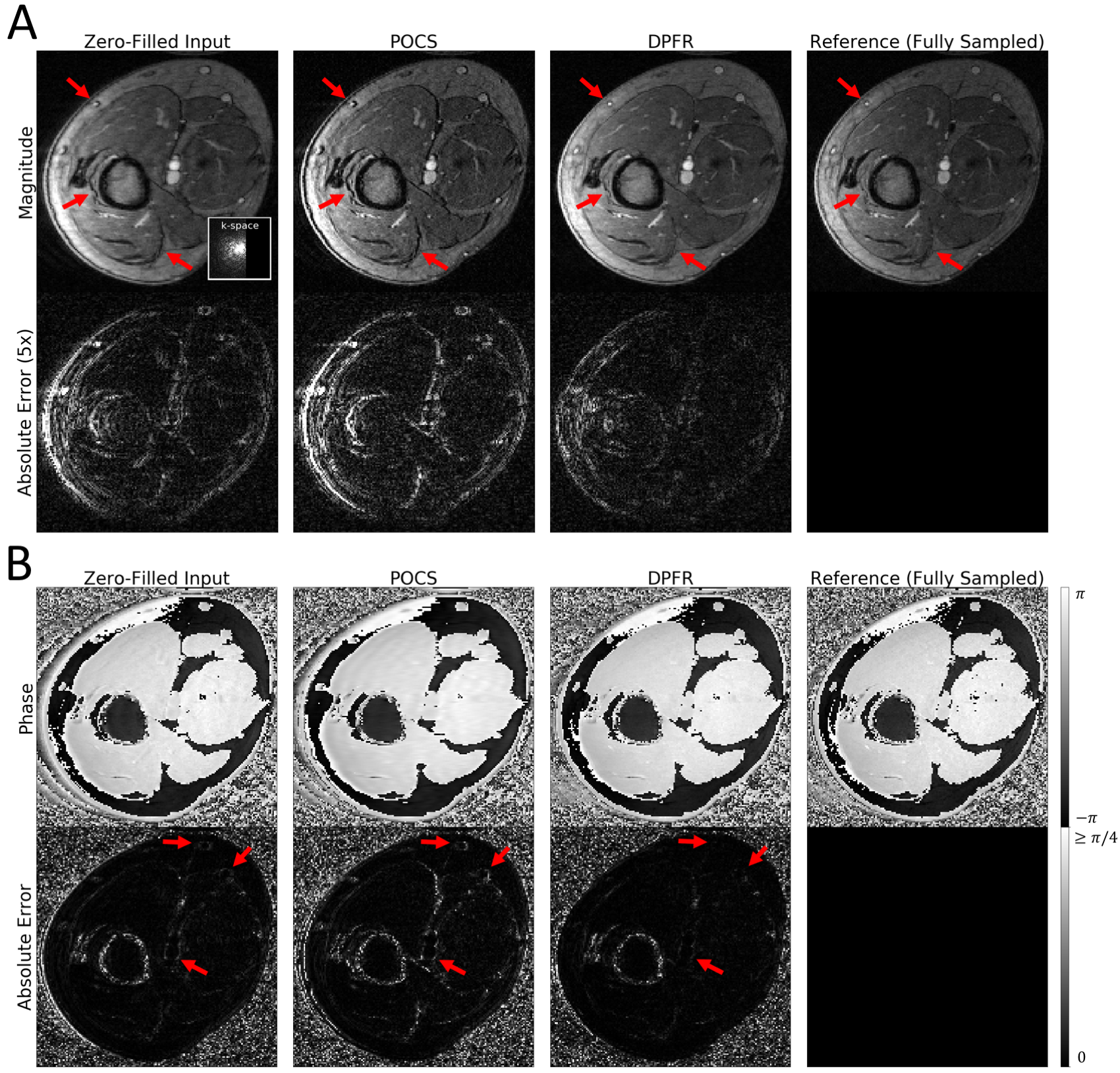
Figure 5. Representative example of partial Fourier reconstruction with zero-filling, POCS, and our DPFR method at PFF=60%, α = 1 (no phase scaling). Complex-valued image outputs are displayed as magnitude (panel A) and phase (panel B). The input image comes from a test exam (not seen during training). Red arrows indicate areas where the different methods vary greatly. Note that residual phase error for DPFR is largely in regions of low signal.