4700
Diffusion-weighted MR Image Reconstruction using Automated Transform by Manifold Approximation (AUTOMAP) on Human Brains1A.A Martinos Biomedical Imaging Center / MGH, Charlestown, MA, United States, 2Harvard Medical School, Boston, MA, United States, 3Department of Physics, Harvard University, Cambridge, MA, United States
Synopsis
Low intrinsic Signal-to-Noise Ratio (SNR) in diffusion-weighted (DW) images are recurrent issues especially at high b-values. Here, we apply the deep neural network image reconstruction technique, AUTOMAP (Automated Transform by Manifold Approximation) to in-vivo diffusion-weighted MR data acquired at 1.5 T with varying b-values. In addition, apparent diffusion coefficient (ADC) maps were assessed. We also compared the reconstruction of the images using two different training corpura. The results for AUTOMAP reconstruction showed a significant increase in SNR.
Introduction
Long scan times and low intrinsic Signal-to-Noise Ratio (SNR) in diffusion-weighted (DW) images are recurrent issues especially at high b-values (b>1000 s/mm2). Various denoising techniques have been developed in the pre or post-processing pipeline to characterize and subtract the noise from the images1,2. Recently a noise-robust image reconstruction approach based on a data-driven learning of the low-dimensional manifold representations of real-world data was described using a deep neural network architecture3. This approach, AUTOMAP (Automated Transform by Manifold Approximation) is an end-to-end automated k-space-to-image-space generalized reconstruction framework that learns a highly-parameterized image reconstruction function optimized for a corpus of training data and is less sensitive to input corruptions. Here, we examine the performance of AUTOMAP for the reconstruction of in-vivo diffusion-weighted MR data acquired at 1.5 T with varying b-values. In addition, apparent diffusion coefficient (ADC) maps were assessed. We also compared the reconstruction of the images using two different training datasets.Materials and Methods
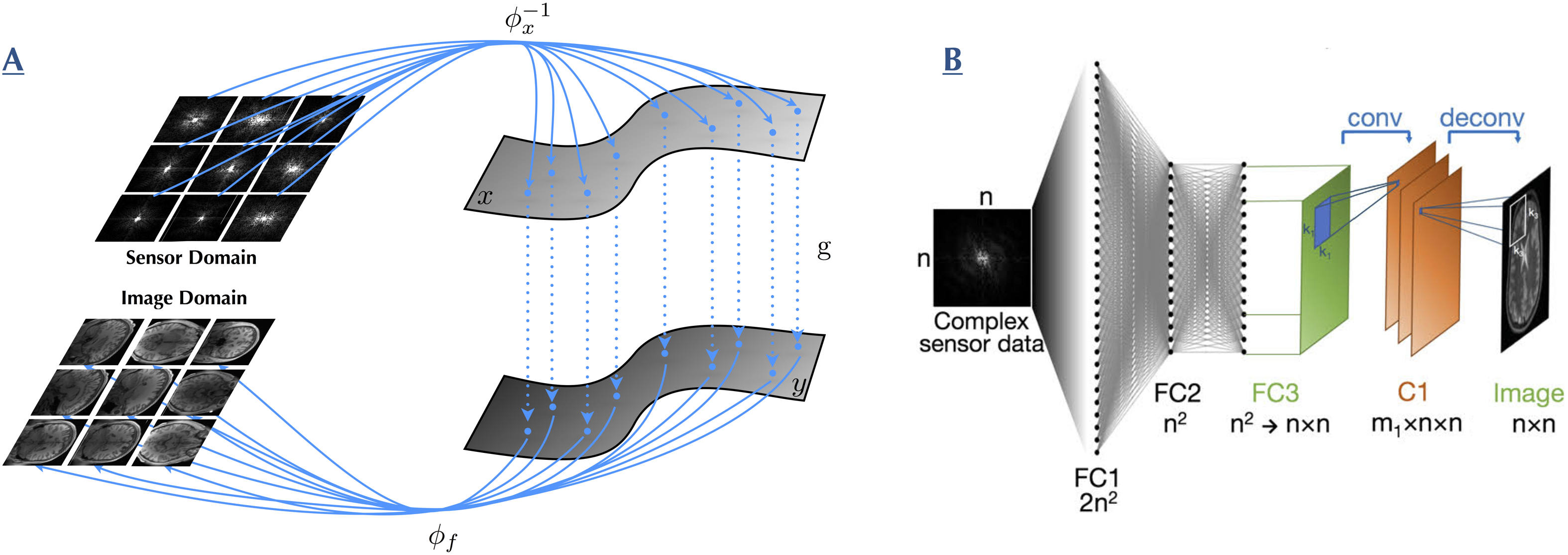
Training set: Two training corpora were assembled 1) from 61,000 2D diffusion-weighted (DW) brain MR images which included b-values ranging from 1000 – 10000s/mm2 and 2) from 51,000 2D T1-weighted (T1-W) brain MR images. Both training corpora were selected from the MGH-USC Human Connectome Project (HCP)4 public database. The images were cropped to 256 × 256 and were subsampled to 128×128, symmetrically tiled to create translational invariance and finally normalized to the maximum intensity of the data. To produce the corresponding k-space representations for training, each image was Fourier Transformed with MATLAB’s native 2D FFT function.
Architecture of NN: The NN was trained to learn an optimal feed-forward reconstruction of k-space domain into the image domain. The real and the imaginary part of datasets were trained separately. The network, described in Figure 1, was composed of 2 fully connected layers (input layer and 1 hidden layer) of dimension n2×1 and activated by the hyperbolic tangent function. The 3rd layer was reshaped to n × n for convolutional processing. One convolutional layer, C1 convolved 64 filters of 5×5 with stride 1 followed by a rectifier nonlinearity. The final output layer deconvolves the C1 layer with 64 filters of 7×7 with stride 1. The output layer resulted into either the reconstructed real or imaginary component of the image.
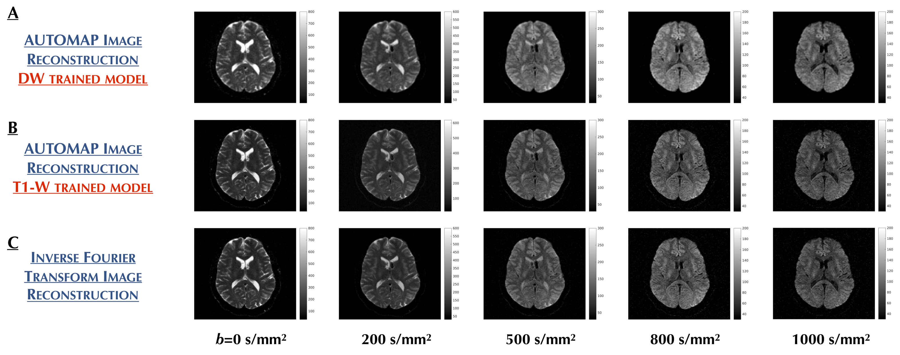
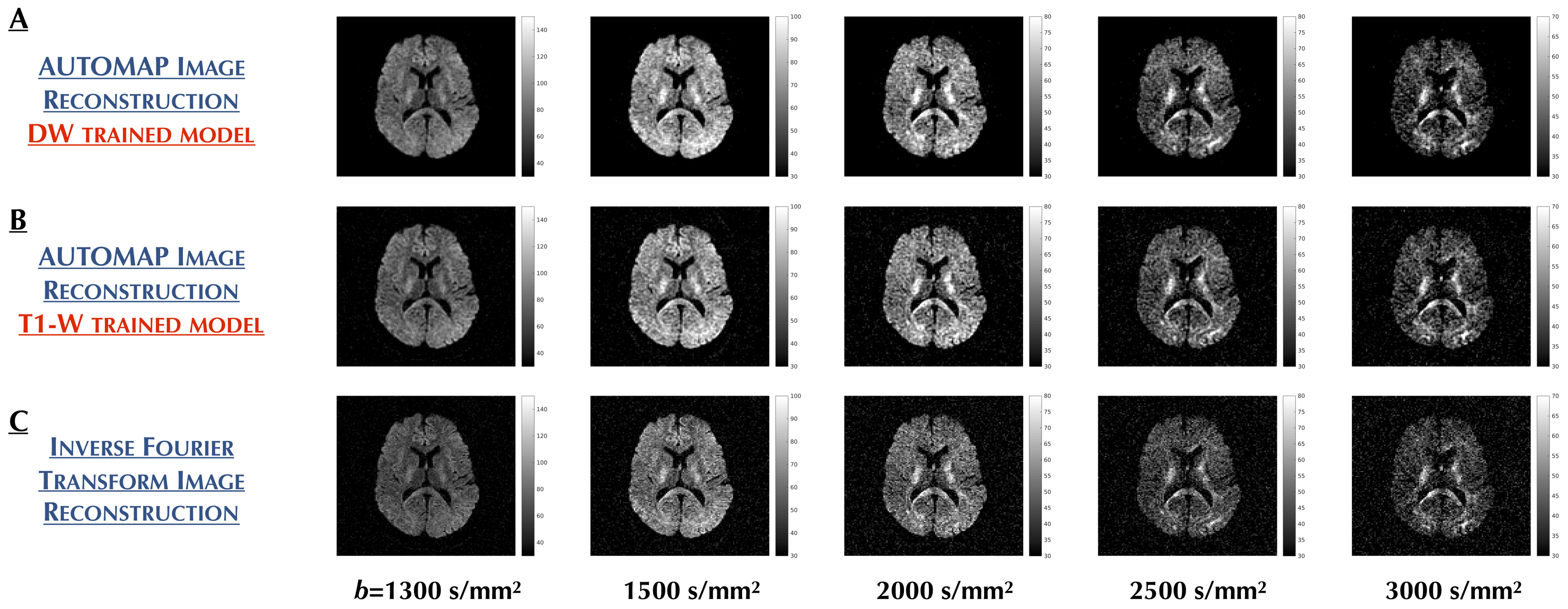
Data Acquisition & Reconstruction: 2D in vivo DW brain images at 1.5 T were acquired with single shot Spin Echo EPI sequence. The sequence parameters were: TR =5000ms, TE = 136ms, TI = 2500ms, matrix size = 128×128, spatial resolution = 1.8mm×1.8mm, a slice thickness = 6.5 mm, number of slices = 24, number of coils = 4 and number of averages (NA) was set to 1. Images were acquired with b-values: 0, 200, 500, 800, 1000, 1300, 1500, 2000, 2500, 3000 s/mm2 and the diffusion gradients were along 3 directions. For AUTOMAP reconstruction, 1 image slice from each coil, each b-value and each direction were Fourier Transformed with MATLAB’s native 2D FFT function and reconstructed using either trained brain models above.
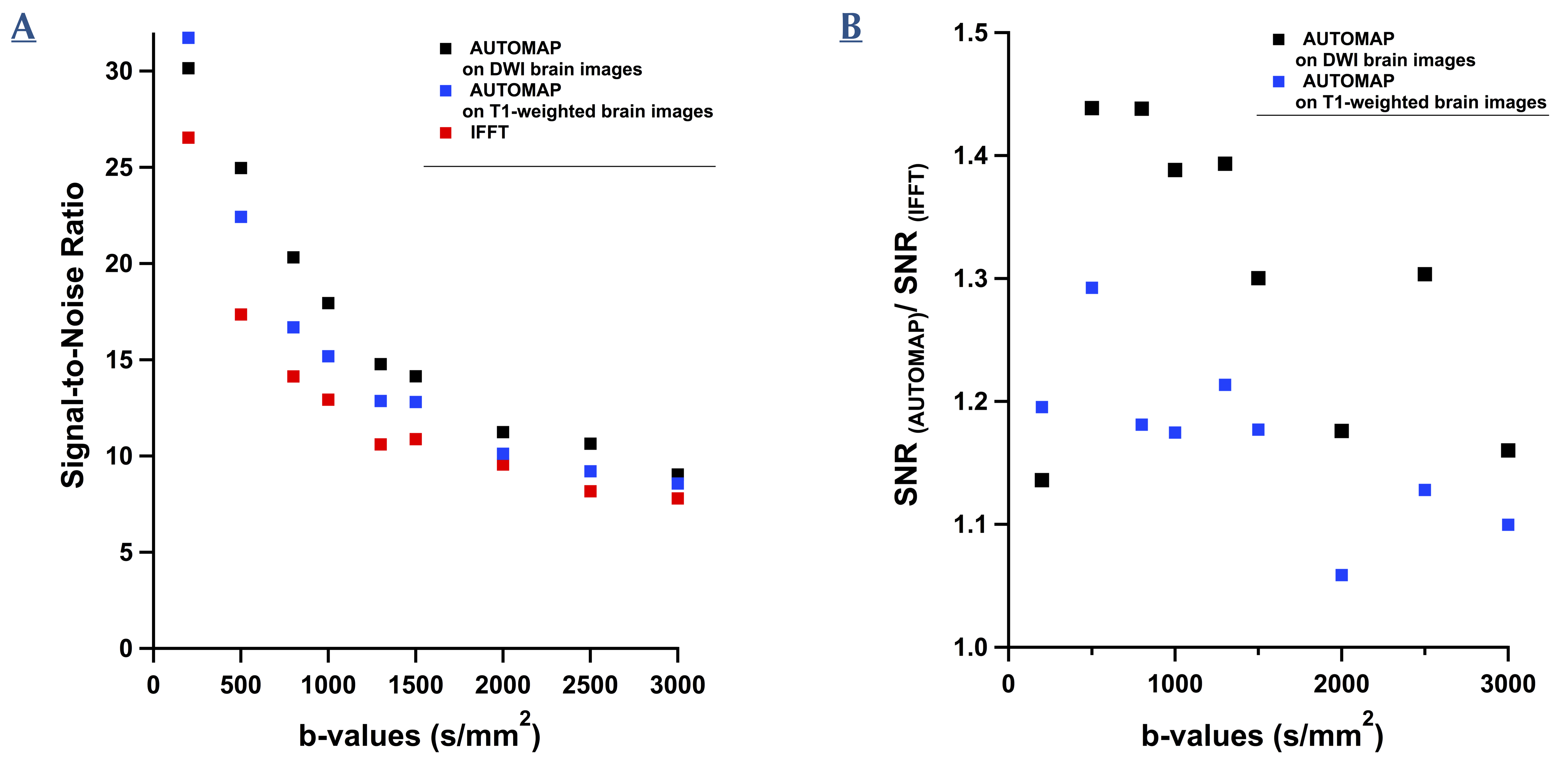
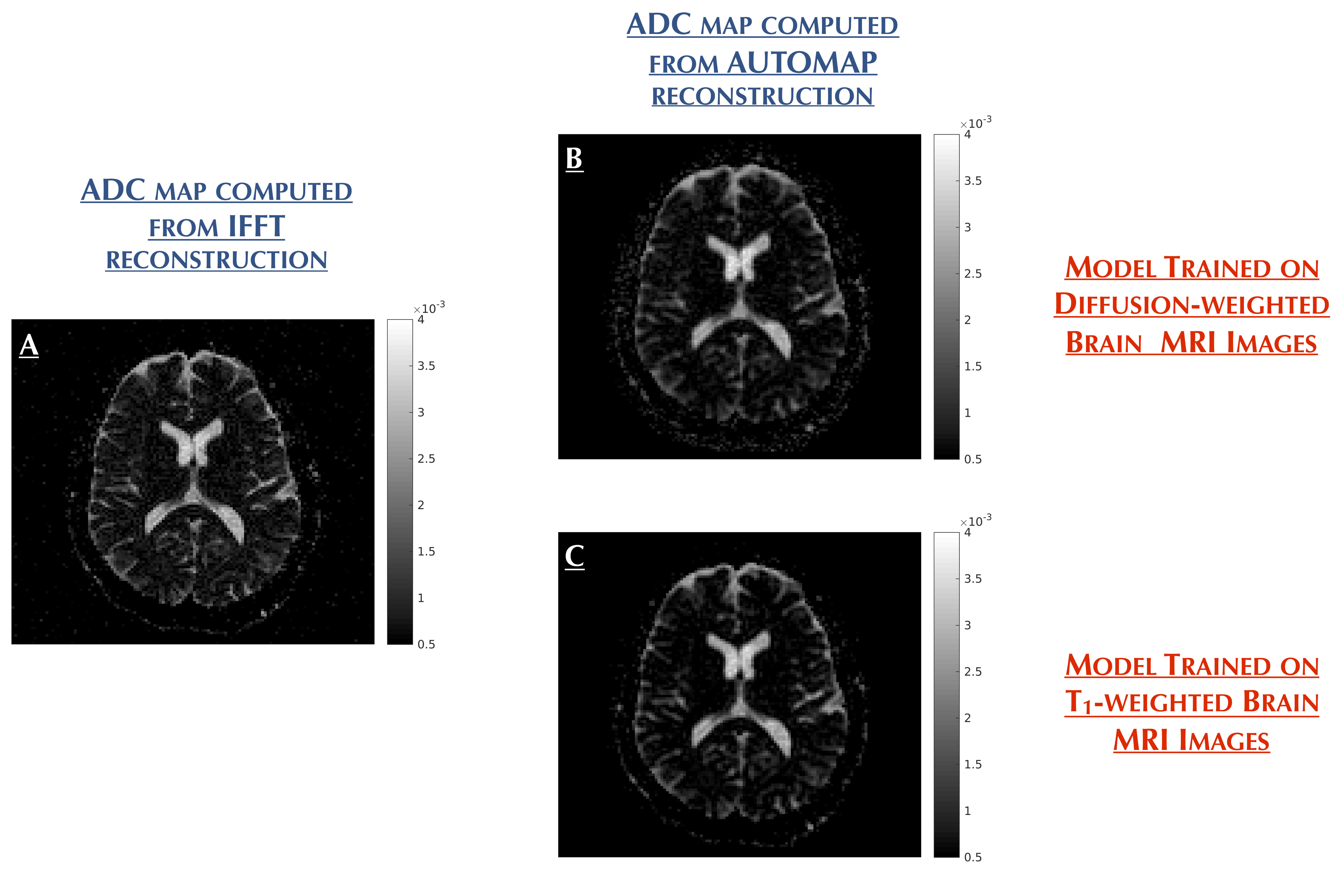
Data Analysis: The signal magnitude of the AUTOMAP reconstructed images were normalized to the scale of the conventional IFFT reconstructions with a constant scalar determined by matching the AUTOMAP and IFFT intensities of the ventricles at b-value=0. SNR was then computed by dividing the signal magnitude by the standard deviation of the noise. The gain in SNR was also calculated by taking the ratios of SNRs of the AUTOMAP reconstructed images over the IFFT reconstructed images. The apparent diffusion coefficient (ADC) maps were also computed with , where , is the signal intensity with the gradient factor b-value=1000 s/mm2 and , the signal intensity with all diffusion-sensitizing gradients turned off.
Results
Figures 2 and 3 shows the performance of AUTOMAP over IFFT reconstruction across the nine b-values using the DW and T1-W trained models respectively. The DW trained model-based reconstruction shows a significant improvement in the SNR (in Figure 4) when compared to the IFFT reconstruction and also compared to the T1-W trained model-based reconstruction. A signal gain of more than 40% has been evaluated for b-value of 1300 s/mm2 and for higher b-values the SNR gain is observed across both trained models. ADC maps for the 2 trained models are in good agreement with that of IFFT.Discussion & Conclusion
The reconstruction performance of AUTOMAP on low SNR data demonstrates the robustness of the reconstruction technique and its high immunity to noise in the ULF regime. Due to lack of correct diffusion coefficient metrics, the quantitative assessment of the ADC maps was not conducted. Future work will include the application of AUTOMAP on real raw in vivo data diffusion weighted datasets without corrections and a deeper assessment on the parametric ADC maps.
Acknowledgements
No acknowledgement found.References
1.Haldar, Justin P et al. “Improved diffusion imaging through SNR-enhancing joint reconstruction” Magnetic resonance in medicine vol. 69,1 (2012): 277-89.
2. F. Lam, S. D. Babacan, J. P. Haldar, N. Schuff and Z. Liang, "Denoising diffusion-weighted MR magnitude image sequences using low rank and edge constraints," 2012 9th IEEE International Symposium on Biomedical Imaging (ISBI), Barcelona, 2012, pp. 1401-1404
3.‘Image reconstruction by domain transform manifold learning’, B. Zhu and J. Z. Liu and S. F. Cauley and B. R. Rosen and M. S. Rosen, Nature 555 487 EP - (2018).
4 ‘MGH–USC Human Connectome Project datasets with ultra-high b-value diffusion MRI’, Fan, Q. et al. NeuroImage 124, 1108–1114 (2016).
Figures