4664
Fast estimation of GRAPPA kernel using Meta-learning1Bio and Brain Eng., KAIST, Daejeon, Korea, Republic of
Synopsis
This paper proposes an accelerated MR reconstruction method for parallel imaging from uniformly undersampled k-space data by learning scan-specific GRAPPA kernel using the long short-term memory network (LSTM). In particular, the meta-leaner LSTM is redesigned to quickly estimate the GRAPPA kernel for each k-space from its auto-calibration signals (ACS). The proposed method shows improved reconstruction performance with minimum error.
Introduction
Recently, inspired by the success of deep learning from computer vision research,1-5 deep learning approaches have been extensively studied for accelerated MR imaging.6-9 Most of the existing deep learning approach for MR reconstruction have focused on improving the average reconstruction performance for all training dataset.6-9 Generalized auto-calibrating partially parallel acquisitions (GRAPPA)10 and Robust artificial-neural-networks for k-space interpolation (RAKI)11 tried to find the scan-specific kernel from its auto-calibration signals (ACS). However, they need separate step to find the scan-specific kernels such as matrix inverse or neural network training process for each scan, which is time-consuming. Here, we propose a meta-learning based algorithm to estimate the scan-specific GRAPPA kernel for parallel imaging using the learner extracted by a Long Short-Term Memory network12(LSTM)-based meta-learner optimizer.
Methods
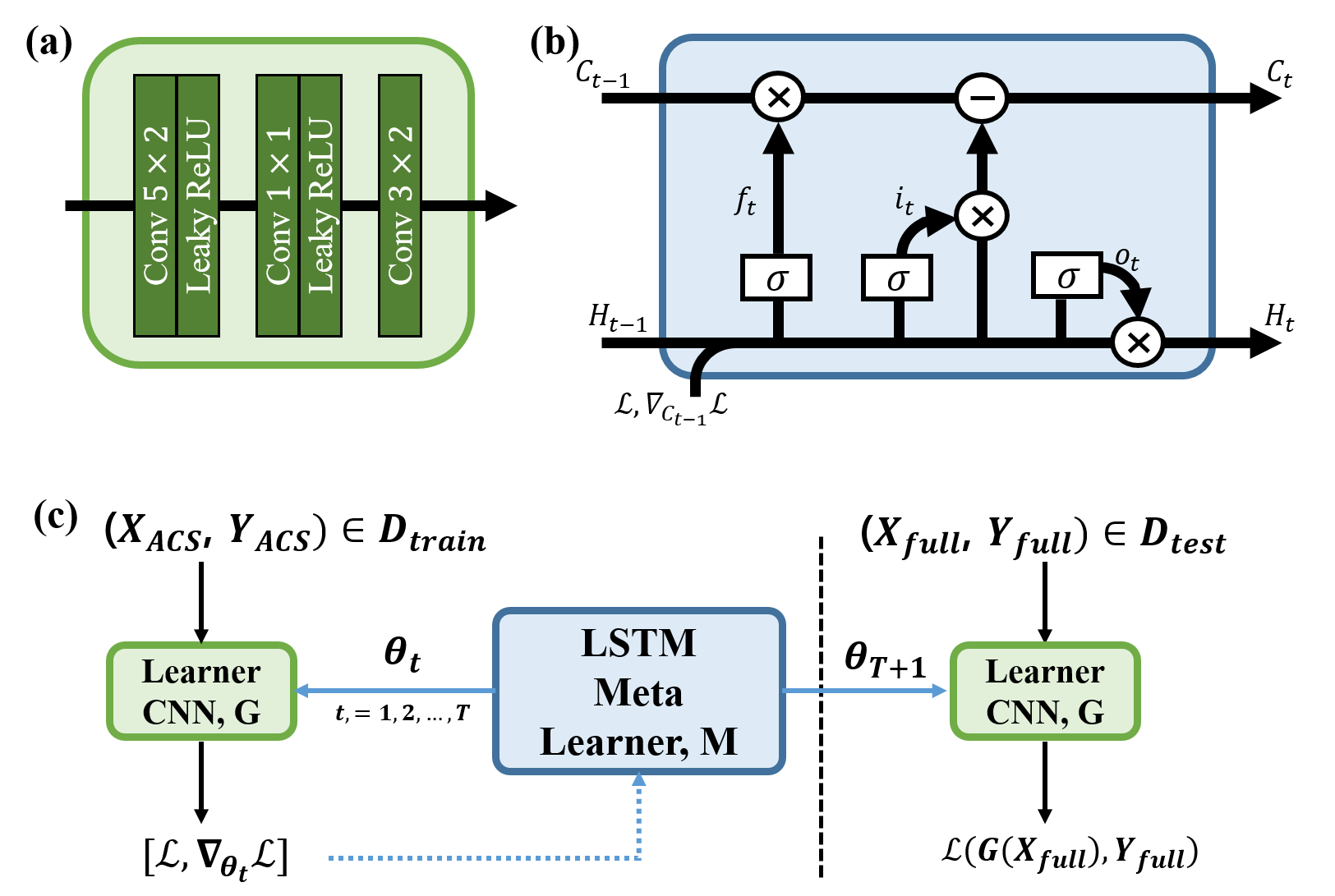
Suppose we train the parameters of a leaner CNN, $$$\theta$$$, using the gradient descent algorithm. The $$$t$$$-th update $$$\theta_t$$$ can be represented by
$$\theta_t=\theta_{t-1}-\alpha\nabla_{\theta_{t-1}}\mathcal{L}$$
where $$$\alpha$$$ and $$$\nabla_{\theta_{t-1}}\mathcal{L}$$$ are the learning rate and the gradients of the loss with respect to $$$\theta_{t-1}$$$, respectively. Ravi, et al.13 observed that the LSTM could be used as an optimization tool because of the similarity between the equations for gradient update and cell states update as following:
$$C_{t}=f_t\odot C_{t-1}+i_t\odot\tilde{C}$$
if $$$C_{t-1}=\theta_{t-1}$$$, $$$f_t = 1$$$, $$$i_t = \alpha$$$ and $$$\tilde{C} = -\nabla_{\theta_{t-1}} \mathcal{L}$$$. The meta-learner LSTM was successfully applied to the few-shot learning task as a powerful acceleration technique for optimization. Moreover, it is also as a provider for good initialization, resulting in great performance on the few-shot classification task.13 The proposed algorithm consists of two neural networks, a learner CNN and a meta-learner LSTM as shown in Fig.1. The learner CNN reconstructs the missing k-space using the sampled k-space as an input. The meta-learner LSTM has modified LSTM structure as shown in Fig.1 (b). The proposed meta-learner LSTM receives the whole weights of the learner CNN, $$$\theta$$$, as a vectorized cell state, $$$C_{t}$$$, and update it as follows:
$$C_{t}=f_t\odot C_{t-1}-i_t\odot(\nabla_{\theta_{t-1}}\mathcal{L}+H_{t-1})$$
where $$$H_{t-1}$$$ is the hidden state of the LSTM. Here, we redesign the output gate as momentum gate to transfer the previous gradients by hidden state. The hidden state, $$$H_t$$$, is updated by the following form:
$$ H_t=o_t\odot(\nabla_{\theta_{t-1}}\mathcal{L}+H_{t-1})$$
where the forget, input and momentum gates are as followings,
$$i_{t}=\sigma(W_i[H_{t-1},\mathcal{L},\nabla_{\theta_{t-1}}\mathcal{L},i_{t-1}]+b_i)$$
$$f_{t}=\sigma(W_f[H_{t-1},\mathcal{L},\nabla_{\theta_{t-1}}\mathcal{L},f_{t-1}]+b_f)$$
$$o_{t}=\sigma(W_o[H_{t-1},\mathcal{L},\nabla_{\theta_{t-1}}\mathcal{L},o_{t-1}]+b_o).$$
The MR dataset was acquired in Cartesian coordinate with 7T MR scanner (Philips, Achieva). The following parameters were used for multi-slice FFE scan: TR 831ms, TE 5ms, slice thickness 0.75mm, 288$$$\times$$$288 matrix, 32 coils, FOV 240$$$\times$$$240mm, and FA 15 degrees. Total 567 number of the axial brain images were scanned from nine subjects. The scans are divided by 7/1/1 subjects for $$$\mathcal{D}_{meta-train}$$$/ $$$\mathcal{D}_{meta-validation}$$$/ $$$\mathcal{D}_{meta-test}$$$, respectively. Each $$$\mathcal{D}_{meta-set}$$$ consists of $$$D_{train}$$$ and $$$D_{test}$$$. We designed two input/target pairs from each k-space. Specifically, $$$(X_{ACS}$$$, $$$Y_{ACS})\in D_{train}$$$ refer to the sampled/missing k-space from ACS, while $$$(X_{full}$$$, $$$Y_{full})\in D_{test}$$$ denotes the sampled/missing k-space from whole k-space. The learner CNN initially reconstructs the k-space from ACS ($$$D_{train}$$$) and the loss function is calculated as following:
$$\mathcal{L}_{train}=||G(\theta_t;X_{ACS})-Y_{ACS}||^2.$$
The loss and the gradients of the loss are fed to the meta-learner LSTM, $$$M$$$, and $$$\theta_{t+1}$$$ are estimated:
$$\theta_{t+1}=M(\mathcal{L},\nabla_{\theta_{t}}\mathcal{L}).$$
After the $$$T$$$ number of LSTM updates, the final estimated parameters, $$$\theta_{T+1}$$$, are applied to reconstruct the full k-space ($$$D_{test}$$$) to minimize the following cost:
$$\mathcal{L}_{test}=||G(\theta_{T+1};X_{full})-Y_{full}||^2.$$
To train the meta-learner LSTM and to find the best initial state, $$$\theta_0$$$, we minimize the summation of $$$\mathcal{L}_{train}$$$ and $$$\mathcal{L}_{test}$$$. The complex values are handled by concatenating real and imaginary values along the channel direction. The preprocessing method14 for gradients and loss is applied for better performance.
Results and Discussion
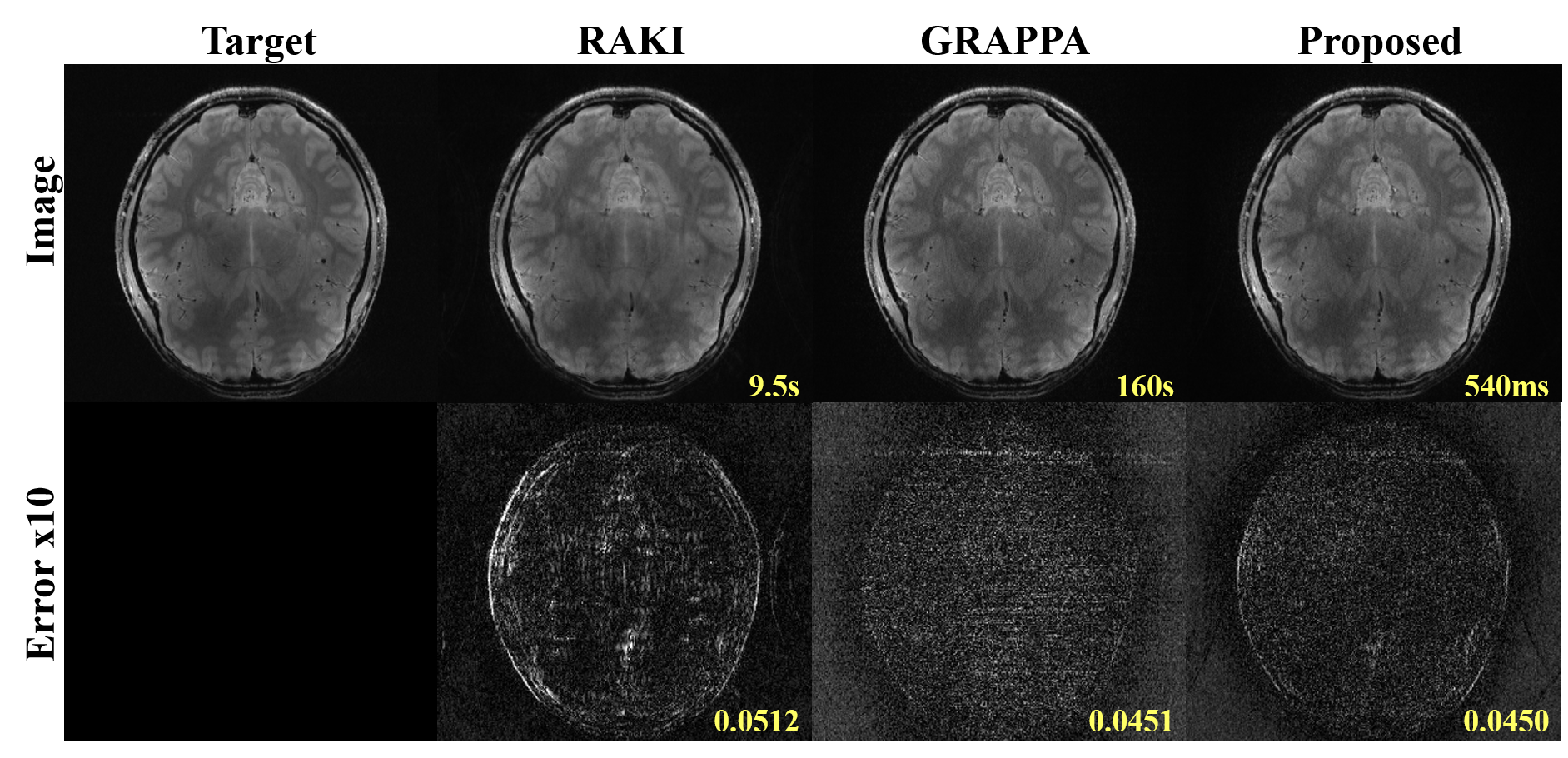
The proposed method shows minimum normalized root mean squared error (NRMSE) compared to RAKI and GRAPPA. The artifacts are still visible in the result of RAKI, when the hyper-parameters are not optimally selected by trial and error. The GRAPPA shows great reconstruction results but the noise from the high-frequency components are amplified. However, the hyper-parameter tuning is not necessary in the proposed method, because it utilizes the LSTM gates as the dynamic hyperparameters. The gates are dynamically tuned at each update for proper and fast optimization based on the current loss, the current gradients, and the previous values of each gate. Accordingly, the proposed method produced the best reconstruction result without high-frequency noise amplification.Conclusion
The proposed method took only 540ms for the reconstruction from 32 coils (Figure 2), which is faster than GRAPPA and RAKI. We presented a fast and scan-specific reconstruction method for the highly under-sampled k-space using LSTM-based meta learner. To our best knowledge, this is the first meta-learning algorithm for accelerated MR imaging.Acknowledgements
This work was supported by Institute for Information & Communications Technology Promotion(IITP) grant funded by the Korea government(MSIT) [2016-0-00562(R0124-16-0002), Emotional Intelligence Technology to Infer Human Emotion and Carry on Dialogue Accordingly]References
1. Krizhevsky A, et al. Imagenet classification with deep convolutional neural networks. In Advances in Neural Information Processing Systems, 2012;1097-1105.
2. Ronneberger O, et al. U-net: Convolutional networks for biomedical image segmentation. In International Conference on Medical Image Computing and Computer-Assisted Intervention, 2015;234-241.
3. Mao X, et al. Image restoration using very deep convolutional encoder-decoder networks with symmetric skip connections. In Advances in Neural Information Processing Systems, 2016;2802-2810.
4. Zhang K, et al. Beyond a Gaussian denoiser: Residual learning of deep CNN for image denoising. IEEE Transactions on Image Processing, 2017;26(7):3142-3155.
5. Dong C, et al. Learning a deep convolutional network for image super-resolution. In European Conference on Computer Vision, 2014;184-199.
6. Kwon K, et al. A parallel MR imaging method using multilayer perceptron. Medical physics, 2017;44(12):6209-6224.
7. Lee D, et al. Deep residual learning for accelerated MRI using magnitude and phase networks. IEEE Transactions on Biomedical Engineering. 2018.
8. Zhu B, et al. Image reconstruction by domain-transform manifold learning. Nature, 2018;555(7697):487.
9. Mardani M, et al. Deep Generative Adversarial Neural networks for compressive sensing (GANCS) MRI. IEEE Transactions on Medical Imaging. 2018.
10. Griswold MA, et al. Generalized autocalibrating partially parallel acquisitions (GRAPPA). Magnetic Resonance in Medicine, 2002;47(6):1202-1210.
11. Wang S, et al. Accelerating Magnetic Resonance Imaging via deep learning. IEEE 13th International Symposium on Biomedical Imaging, 2016;514-517.
11. Akçakaya M, et al. Scan-specific robust artificial-neural-networks for k-space interpolation (RAKI) reconstruction: Database-free deep learning for fast imaging. Magnetic Resonance in Medicine. 2018.
12. Hochreiter S, et al. Long short-term memory. Neural computation, 1997;9(8):1735-1780.
13. Ravi S, et al. Optimization as a model for few-shot learning. International Conference on Learning Representations, 2017.
14. Andrychowicz M, et al. Learning to learn by gradient descent by gradient descent. In Advances in Neural Information Processing Systems, 2016;3981-3989.
Figures