4662
Accelerated 3D Non-Cartesian Reconstruction with Deep Learning1Electrical Engineering, Stanford University, Stanford, CA, United States, 2Electrical Engineering and Computer Sciences, University of California, Berkeley, CA, United States, 3Radiology, Stanford University, Stanford, CA, United States
Synopsis
In this work, we demonstrate the application of a non-Cartesian unrolled architecture in reconstructing images from undersampled 3D cones datasets. One shown application of this method is for reconstructing undersampled 3D image-based navigators (iNAVs), which enable monitoring of beat-to-beat nonrigid heart motion during a cardiac scan. The proposed non-Cartesian unrolled network architecture provides similar outcomes as l1-ESPiRIT in one-twentieth of the time, and the reconstructions exhibit robustness when using an undersampled 3D cones trajectory.
Introduction
Recently, deep
learning techniques have been used to reconstruct k-space data in an accelerated fashion by training neural networks
that take k-space measurements as
inputs and output reconstructed images. Previous approaches such as variational
networks have incorporated model-based ideas for deep reconstruction [1]. Among
these approaches, unrolled network (UN) architectures [2, 3] have been proposed to
reconstruct images by unfolding the reconstruction optimization problem [4]
and learning the regularization functions and coefficients. Prior studies
leveraging UNs have been limited to contexts involving Cartesian
acquisitions. For reconstruction of non-Cartesian datasets, only image-to-image
convolutional neural networks (CNNs) have been investigated [5]. In this work, we
modify the UN to accommodate non-Cartesian datasets and demonstrate
application of the non-Cartesian unrolled architecture in reconstructing images
from undersampled 3D cones datasets.Methods
Neural Network Architecture
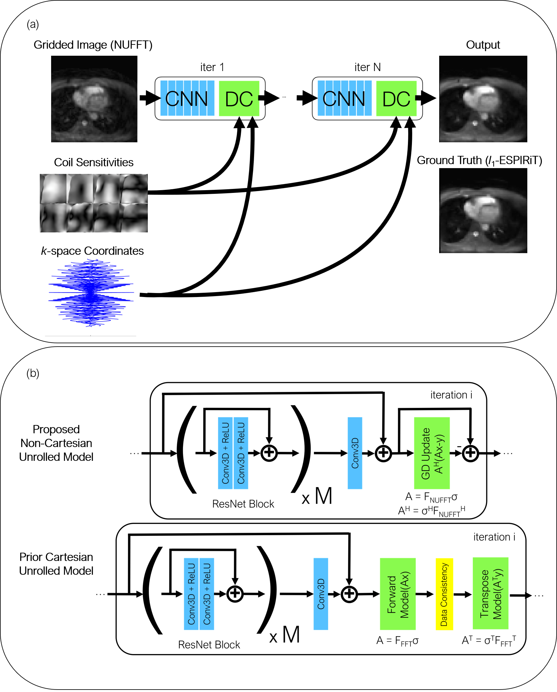
The UN is based on the iterative soft-shrinkage algorithm (ISTA) [4], which solves the following inverse problem with image x, k-space data y, encoding operator A, and regularization term R(x):$$\underset{x}{\text{minimize }}\left\| Ax-y \right \|^2_2 + R(x)$$ The solution, which is found using proximal gradient descent, iterates between the shrinkage thresholding and data consistency steps:$$x^{k+1} = S_R(x^k - A^T(Ax^k - y))$$ When using non-Cartesian data, acquisition model A incorporates coil sensitivity maps computed using ESPIRiT [6], and the non-uniform FFT (NUFFT) operator. Note that in prior usages of the UN for Cartesian datasets, the acquisition model applied an FFT. The regularization term is implicitly learned by replacing its proximal operator SR with a CNN.
The UN architecture uses 5 gradient steps (iterations) consisting of 2 residual network (ResNet) [7] blocks per step. The input into the network is the undersampled 3D k-space data, k-space coordinates (to generate the NUFFT operator), and the respective coil sensitivity maps for each channel. The ground truth for training is the undersampled dataset reconstructed with l1-ESPIRiT [6]. The input into each gradient step is comprised of coil-combined image-space data (transpose NUFFT operator applied to the k-space data) after performing SENSE reconstruction [8]. Each ResNet block uses two 3D convolutional layers with a kernel size of 3x3x5 and filter depth of 128 followed by a ReLU activation function. An additional layer is added to the end of each unrolled step which outputs 2 channels (real and imaginary) for the k-space data. The final layer is added to a skip connection from the input of the first ResNet block to accelerate training convergence. The data is then converted back to k-space for the data consistency step described above and the gradient step block is repeated 4 more times (5 total). The proposed architecture (Figure 1) was implemented in Python with TensorFlow.
Training Data
One application of this method is for reconstructing 3D image-based navigators (iNAVs), which enable monitoring of beat-to-beat nonrigid heart motion during a cardiac scan. Using an undersampled 3D cones trajectory, a cardiac-triggered low-resolution 3D image of the heart can be collected every heartbeat (28x28x14 cm3 FOV, 4.4 mm isotropic spatial resolution, 176 ms temporal resolution). The reconstruction requirements are substantial as each scan involves the collection of several hundred 3D iNAVs.
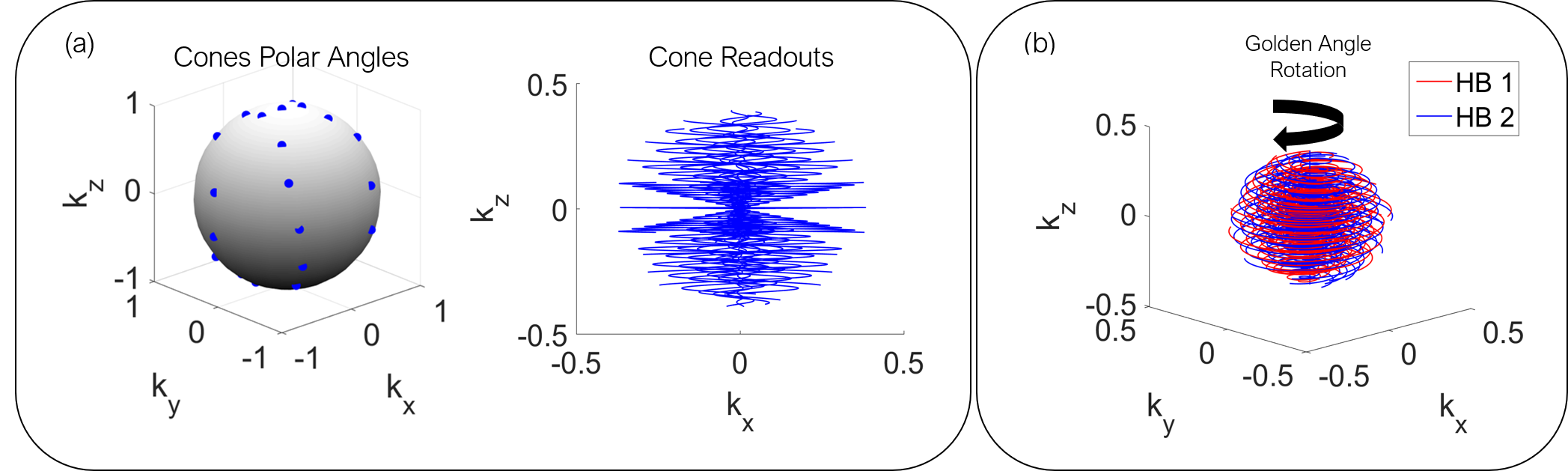
For training, we collected 500 3D iNAVs on a 1.5T GE Signa system with an 8-channel cardiac coil [9]. Specifically, 500 cardiac datasets were acquired separately in different heartbeats using a variable density conical trajectory consisting of 32 readouts, which corresponds to an acceleration factor of 9. Also, an additional 500 datasets were acquired with the same trajectory rotated by the golden angle between each heartbeat to improve further generalization of the model with different k-space sampling patterns. More details for both trajectories are shown in Figure 2.
Results and Discussion
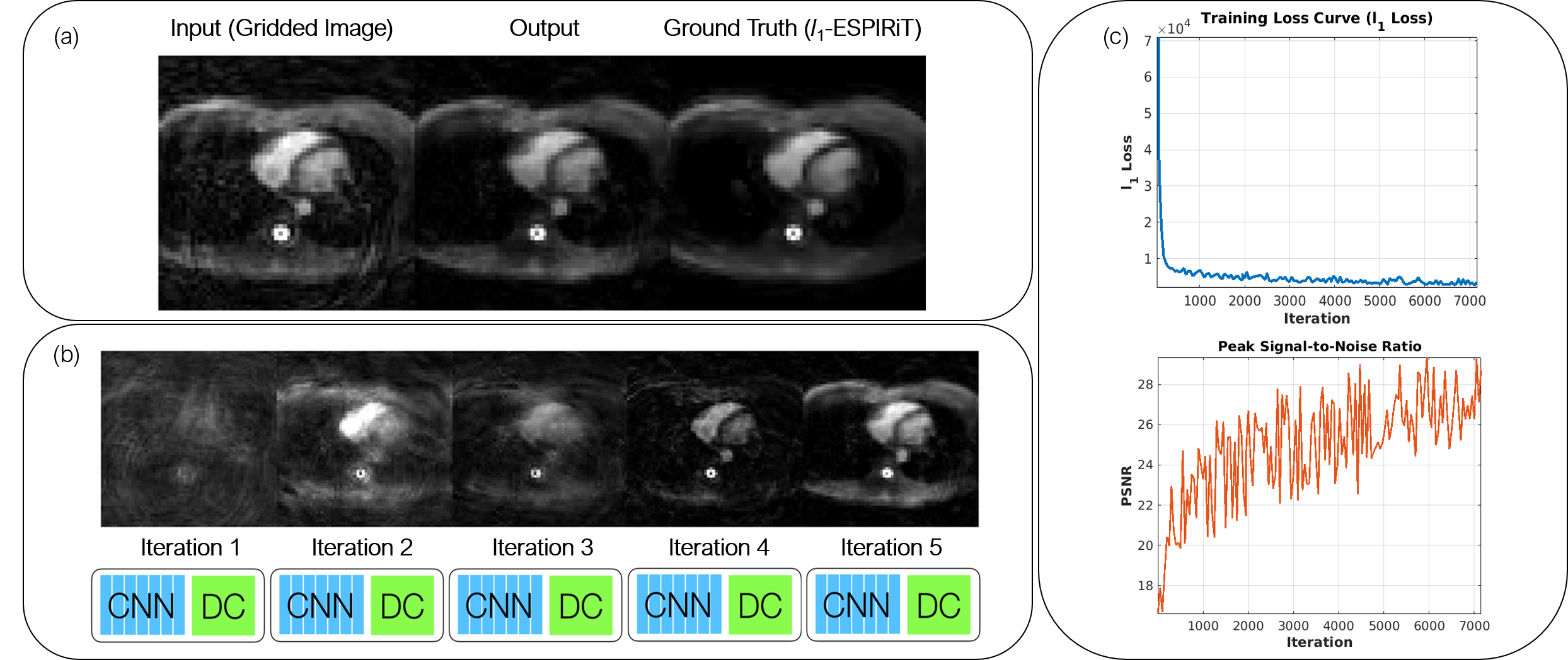
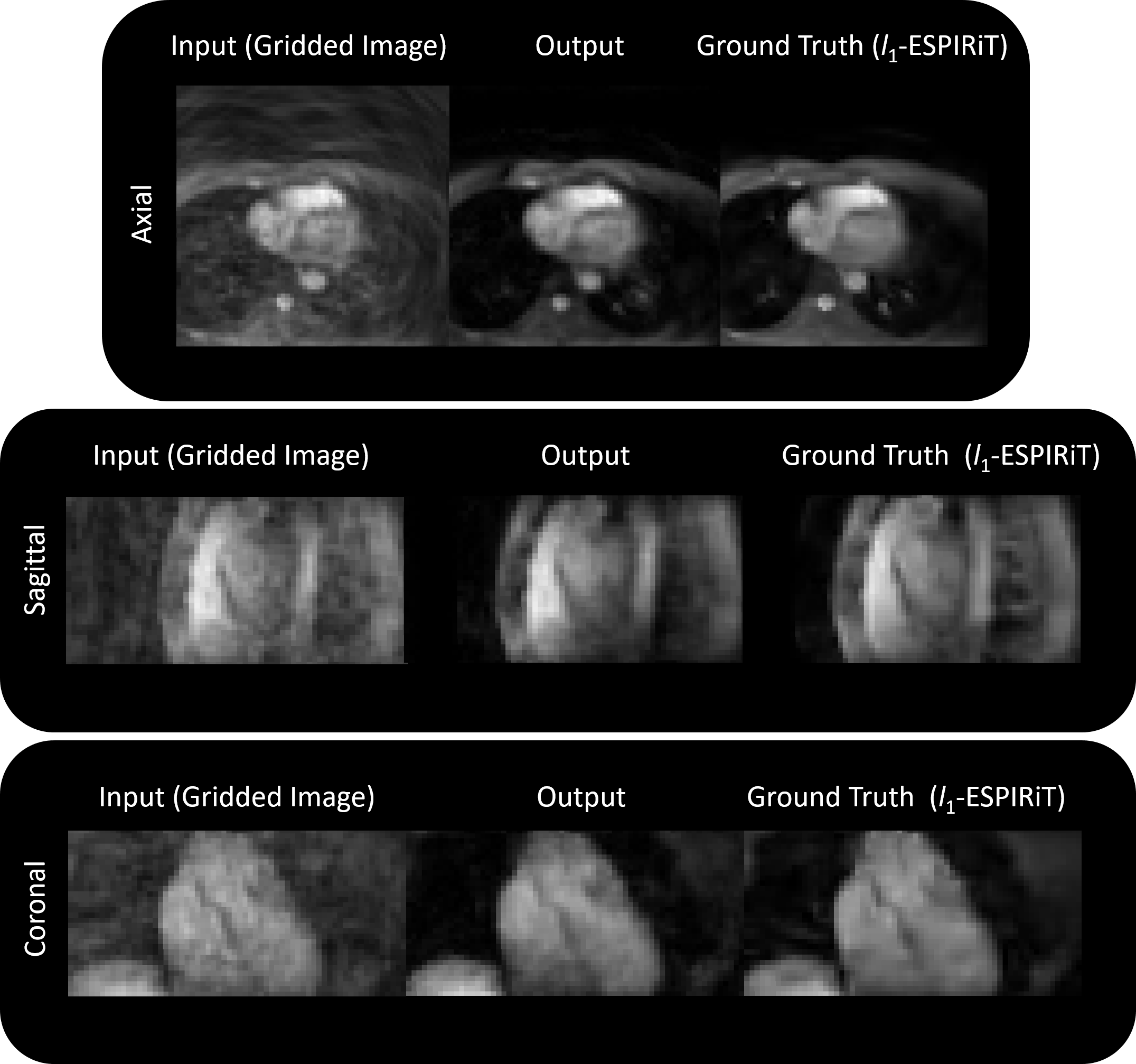
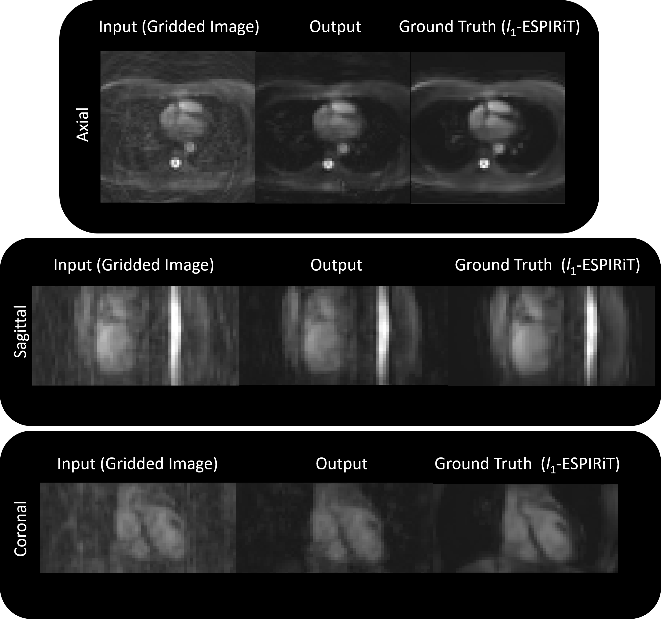
An example input (gridded image), output, and ground truth (after l1-ESPIRiT) is shown in Figure 3a and the respective outputs for each iteration (gradient step) are shown in Figure 3b. When using the l1 loss, the training error converged quickly and peak signal-to-noise ratio (PSNR) gradually increased (Figure 3c). When employing the trained architecture, the undersampled cardiac images (compared to the outcomes from gridding) retained structural features as a result of the denoising/smoothening operation. More specifically, aliasing artifacts arising from undersampling a cones trajectory were effectively removed after evaluation by the network. Output images from testing the model with unseen datasets are shown in Figures 4 and 5. Inference time for the proposed architecture is 1 second per dataset, while l1-ESPiRIT requires approximately 20 seconds.
The proposed non-Cartesian UN architecture provides similar outcomes as l1-ESPiRIT in one-twentieth of the time. We have shown that the proposed non-Cartesian UN exhibits robustness when using an undersampled 3D cones trajectory.
Acknowledgements
We gratefully acknowledge the support of NIH grants R01HL127039, T32HL007846, and the National Science Foundation Graduate Research Fellowship under Grant No. DGE-114747.
References
[1] Hammernik, Kerstin, et al. "Learning a variational network for reconstruction of accelerated MRI data." Magnetic Resonance in Medicine 79.6 (2018): 3055-3071.
[2] Diamond, Steven, et al. "Unrolled Optimization with Deep Priors." arXiv preprint arXiv:1705.08041 (2017).
[3] Cheng, Joseph Y., et al. "Highly Scalable Image Reconstruction using Deep Neural Networks with Bandpass Filtering." arXiv preprint arXiv:1805.03300 (2018).
[4] Daubechies, Ingrid, et al. "An iterative thresholding algorithm for linear inverse problems with a sparsity constraint." Communications on Pure and Applied Mathematics: A Journal Issued by the Courant Institute of Mathematical Sciences 57.11 (2004): 1413-1457.
[5] Hauptmann, Andreas, et al. "Real‐time cardiovascular MR with spatio‐temporal artifact suppression using deep learning–proof of concept in congenital heart disease." Magnetic Resonance in Medicine (2018).
[6] Uecker, Martin, et al. "ESPIRiT — an eigenvalue approach to autocalibrating parallel MRI: where SENSE meets GRAPPA." Magnetic Resonance in Medicine 71.3 (2014): 990-1001.
[7] He, Kaiming, et al. "Deep residual learning for image recognition." Proceedings of the IEEE Conference on Computer Vision and Pattern Recognition. 2016.
[8] Pruessmann, Klaas P., et al. "SENSE: sensitivity encoding for fast MRI." Magnetic Resonance in Medicine 42.5 (1999): 952-962.
[9] Addy, Nii Okai, et al. "3D image‐based navigators for coronary MR angiography." Magnetic Resonance in Medicine 77.5 (2017): 1874-1883.
Figures