4658
A Reference-Free Convolutional Neural Network Model for Magnetic Resonance Imaging Reconstruction from Under-Sampled k-Space1Shanghai Key Laboratory of Magnetic Resonance, East China Normal University, Shanghai, China, 2MR Scientific Marketing, Siemens Healthcare, Shanghai, China, 3Shanghai University of Medicine & Health Sciences, Shanghai, China
Synopsis
We used a reference-free model based on convolutional neural network (RF-CNN) to reconstruct the under-sampled magnetic resonance images. The model was trained without fully sampled image (FS) as the reference. We compared our model with the traditional compressed sensing reconstruction (CS) and the CNN model trained by FS. Mean square error and structure similarity were used to evaluate the model. Our RF-CNN model performed better than CS, but did not perform as good as usual CNN model.
INTRODUCTION
Random sampling with compressed sensing (CS) reconstruction can shorten the scanning time of magnetic resonance imaging (MRI). Recently, Convolutional neural networks (CNN) were used on MRI reconstruction from under-sampled k-space to shorten the reconstruction time compared to CS1. However, in some clinical cases such as cardiovascular imaging, it is hard to acquire fully-sampled high-quality images (FS) for training the CNN model. Here we proposed a reference-free CNN model (RF-CNN) without FS to reconstruct the under-sampled k-space.METHODS
We used the T1W image from MIDAS dataset (resolution=1x1x1 mm3) in this work2. We separated the dataset to three groups: training data set (88 cases, 9888 slices), validation data set (4 cases, 432 slices), and testing data set (5 cases, 540 slices). All images in the training dataset were augmented with random zooming, shifting, rotating and shearing. Then we cropped all images to the size of 192x192 and normalized them by subtracting mean value and dividing by the standard deviation. A pseudo-randomly sampling (rate=40%) mask was designed to under-sample the k-space data. We applied Fourier transform (FT) on the images and extracted the k-space data according to the sampling mask. We filled zero in the unsampled position in k-space to match the sampling matrix size. Inverse FT was applied to get zero-filling reconstruction (ZF). We showed the FS, sampling mask, and ZF in Figure 1.
We used a U-Net based 2D model named RF-CNN to reconstruct the MR images (Figure 2)3. We input ZF into the model and get the output of U-Net based model to get the reconstructed image. Then FT was applied on the output to get the reconstructed k-pace. We calculated the mean square error (MSE) between the full sampled k-space and the corresponding reconstructed k-space and used this value as the loss function of the model. However, the usual image-out network used the MSE calculated between the reconstructed image and the FS image as the loss function.
During the training, we used Adam algorithm to minimize the loss function. Some tricks such as learning rate reducing and early stopping were used to increase the efficiency of the training. All processes above were implemented with TensorFlow 1.114 and Python 3.5.
We compared the reconstruction accuracy among our RF-CNN model, the image-out CNN model that trained by minimizing the MSE reference to FS, and the compressed sensing (CS) reconstruction by Split Bregmam Algorithm5. We used MSE and structure similarity (SSIM) to quantify the performance. Paired t-test was used for statistics.
Results
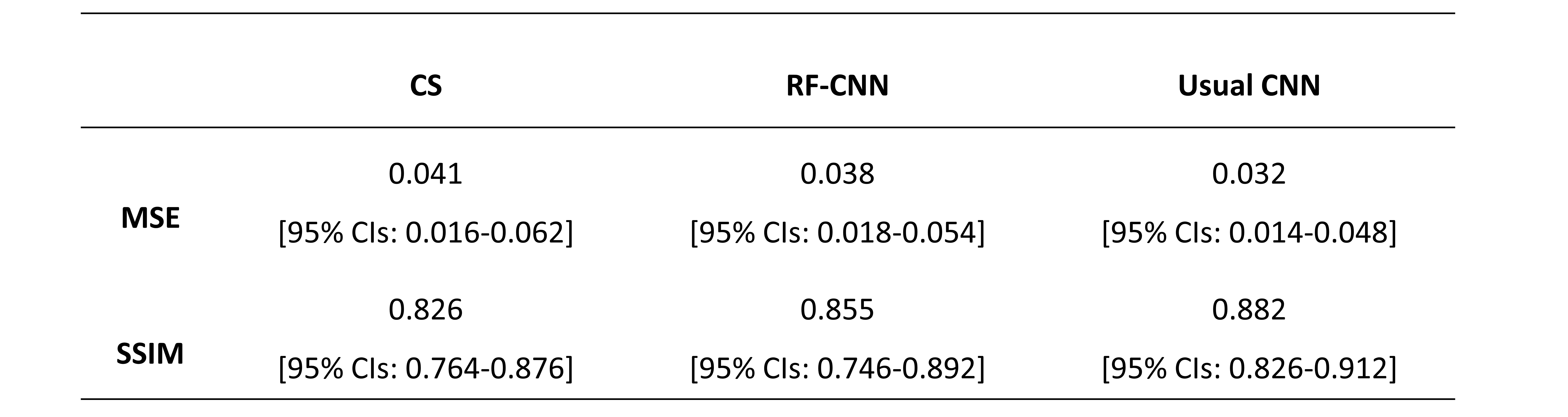
We showed one slice of CS reconstruction, CNN reconstruction and RF-CNN reconstruction in Figure 3, respectively. CNN outperformed the CS and RF-CNN. The quality of RF-CNN is similar to the quality of CS reconstruction. We applied statistics on the MSE and SSIM of total 540 slices of 5 cases in testing data set. The mean value and the 95% confidence intervals (95% CIs) were calculated in Table 1. RF-CNN showed better reconstruction than the CS reconstruction (MSE: p<0.0001, SSIM p<0.001). The reconstruction time for each slice of CS is more than 1 second and that of RF-CNN is only about 10ms.
We also plotted the MSE of the validation data set against the iterative epoch during the training process in Figure 4. The training of RF-CNN converged more quickly than the standard CNN, while the iteration reach plateau the common CNN showed smaller MSE than RF-CNN.
Discussion
Although the RF-CNN reconstruction is not as good as the usual CNN reconstruction, RF-CNN reconstruction can reduce the artifacts without the fully sampled image, which used similar process as the compressed sensing. In the former part of RF-CNN model, the max-pooling process behaves similarly to transforming the image into the specific domain (like wavelet or total variant). Meanwhile, the hidden layers with the minimum size are trained to constrain the sparsity of transformed image, and the latter part of the RF-CNN model transforms the data inversely to the reconstruction. We finally used the MSE of the real sampled k-space data as the loss of the model, which can constrain the consistency of the sampled data.CONCLUSION
We proposed a RF-CNN model only trained by under-sampled k-space data. We proved that this model performance comparable to CS reconstruction. But RF-CNN can reconstruct the MR images much faster than the CS reconstruction. The proposed model has potential for the MR image reconstruction in which it is difficult to get the high quality and full-sample MR images.Acknowledgements
This project is supported by National Natural Science Foundation of China (61731009, 81771816)References
1. Wang S, Su Z, Ying L, et al. Accelerating magnetic resonance imaging via deep learning[C]//Biomedical Imaging (ISBI), 2016 IEEE 13th International Symposium on. IEEE, 2016: 514-517.
2. Bullitt E, Zeng D, Gerig G, et al. Vessel tortuosity and brain tumor malignancy: A blinded study. Academic Radiology, 2005, 12:1232-1240
3. Ronneberger O, Fischer P, Brox T, U-Net: Convolutional Networks for Biomedical Image Segmentation, ArXiv, 2015: 1505.04597
4. Abadi M, Barham P, Chen J, et al. Tensorflow: a system for large-scale machine learning[C]//OSDI. 2016, 16: 265-283.
5. Goldstein T, Osher S. The split Bregman method for L1-regularized problems[J]. SIAM journal on imaging sciences, 2009, 2(2): 323-343.
Figures