Synopsis

A variational neural network for the reconstruction of compressed sensing 4D flow MRI is presented. Nine iterations of an iterative reconstruction are unfolded in a neural network which was trained using eight retrospectively undersampled datasets. A phase-invariant network architecture was designed with two types of filter operations, one with equal real and imaginary component and the other operating on image magnitude only. The method is shown to outperform spatial regularization in the Wavelet domain. A retrospectively undersampled patient scan demonstrates that the network can reconstruct pathologies based on healthy training samples. Reconstruction of prospectively undersampled 4D flow MRI shows good agreement of peak velocities and peak flow.

Introduction

Scan times in 4D flow MRI are considerable, hampering the use of the method in clinical routine. With the advent of compressed sensing (CS)¹ and low-rank modelling^2,3 scan times have been reduced, but only at the cost of an increase in reconstruction times which require clinicians to wait several minutes up to hours for the results. Moreover, to enable high undersampling factors, modern CS methods^2,4,5 employ temporal correlations which can lead to underestimation of peak velocities. Unrolling iterative reconstruction methods using neural networks⁶ enables immediate reconstruction of CS acquisitions once the network is trained and promises improved results over standard methods.

In this work, loop unrolling with adaptive filters was implemented and applied to 4D flow MRI. To this end, a phase-invariant network architecture was designed with two sets of filters, one independently filters real and imaginary component and the other operates on image magnitudes. Only spatial regularization was considered due to limited availability of training datasets, their high heterogeneity in terms of sequence parameters and noise.

Methods

FlowNet

Following^6,7 we define the reconstruction network layers via unrolling$$$\;k=9\;$$$iterations of the gradient descent (GD) algorithm with$$$\;N_f=15\;$$$filters that are applied on complex-valued and magnitude images:

$$\mathbf{x}^{(k+1)}\leftarrow \mathbf{x}^{(k)}-\alpha^{(k)}\mathbf{F}^{\mathtt{H}}\text{diag}(\mathbf{m})(\mathbf{F}\mathbf{x}^{(k)}-\mathbf{y}) - \sum_{i\leq N_f}\Big[\mathbf{D}_{i,k,1}^{\mathtt{T}}\varphi_{i,k,1}(\mathbf{D}_{i,k,1}\text{Re}(\mathbf{x}^{(k)}))+ \mathbf{D}_{i,k,1}^{\mathtt{T}}\varphi_{i,k,1}(\mathbf{D}_{i,k,1}\text{Im}(\mathbf{x}^{(k)}))+\text{sgn}(\mathbf{x^{(k)}})\odot\mathbf{D}_{i,k,2}^{\mathtt{T}}\varphi_{i,k,2}(\mathbf{D}_{i,k,2}\lvert\mathbf{x}^{(k)}\rvert) \Big]$$

where $$$\mathbf{y}$$$ is the zero-filled k-space for given velocity encoding and cardiac phase, $$$\mathbf{D}_{i,j,k}$$$ are convolution matrices defined by kernels of size $$$n_p=5\times5\times5$$$, $$$\alpha^{(k)}$$$ are the GD step lengths, and $$$\varphi_{i,j,k}$$$ are potential functions parametrized by linear interpolation of $$$n_i=35$$$ reference values $$$\phi_{ijk}\in\mathbb{R}^{n_i}$$$ placed on a uniform grid. The reconstruction model is then defined by the set of parameters

$$\Theta=\left\{\alpha^k,\bf{D}_{i,j,k},\phi_{i,j,k}\right\} _{i,j,k}$$

which is tuned via stochastic optimization of weighted reconstruction errors over the training set $$$\mathcal{T}$$$ and the set of undersampling masks $$$\mathcal{M}$$$ :

$$\min_{\Theta}\mathop{\mathbb{E}}_{\{\mathbf{x}^{\text{gt}},\mathbf{y}\}\in\mathcal{T},\mathbf{m}\in\mathcal{M}}\sum_{k\leq K}\|\mathbf{x}_\Theta^{(k)}(\mathbf{y},\mathbf{m})-\mathbf{x}^\text{gt} \|_1\exp(k-K)\tag{*}$$

During initial experiments we observed that such exponential weighting improves training convergence and effectively constrains the admissible set of reconstruction architectures, thus improving generalization ability of the learned solution.

To minimize (*) we performed$$$\;5*10^{-4}\;$$$iterations of the Adam algorithm⁸ with learning rate$$$\;10^{-3}\;$$$and batch size 2. Kernels of$$$\;\mathbf{D}_{i,j,k}\;$$$are ensured to be zero-centered unit-norm via reparametrization.

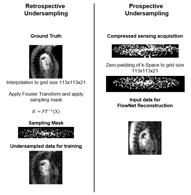
Datasets

Data processing for retrospectively and prospectively undersampled data is illustrated in Figure 1. The training set consists of flow data acquired in the aorta of 8 healthy subjects using a 3T Philips Ingenia system (Philips Healthcare, Best, the Netherlands) using either parallel imaging⁹ or CS¹⁰ for an accelerated acquisition. Spatial and temporal resolution were 2.5x2.5x2.5 mm³ and 25 cardiac phases and encoding velocity was set to 150 cm/s. Data were interpolated on a grid size of 113x113x21, yielding 800 3D complex-valued images which were retrospectively undersampled with 800 variable density CS sampling masks and an acceleration factor of R=6.

Another dataset of a healthy subject acquired with parallel imaging was retrospectively undersampled with acceleration factors of 4, 6 and 8 and a dataset of a patient with dilation of the ascending aorta and combined aortic stenosis and regurgitation due to a bicuspid aortic valve was retrospectively undersampled with R=4.

Prospectively undersampled flow in the aorta of a healthy volunteer was acquired with a pseudo-radial Cartesian spiral sequence and data-driven respiratory motion detection and R=4. The coil dimension was reduced to 5 channels using geometric coil compression¹¹ and the coil channels were reconstructed separately and combined¹². For comparison, 4D flow MRI was also measured and reconstructed with a standard parallel imaging protocol⁹.

Compressed Sensing Reconstruction

As a baseline for comparison, the data were reconstructed using standard CS reconstruction with spatial regularization and Daubechies-4 wavelets as sparse transform (CS-Wavelet).$$\widehat{x}=\min_x ||F^HF(x)-y||_2^2 + \lambda ||\Psi x||_1.$$

Results

Reconstruction time was 0.12 seconds per 3D volume, leading to 12 seconds reconstruction time for the retrospectively undersampled data and 1 minute for the prospectively undersampled data with 5 separate coil channels.

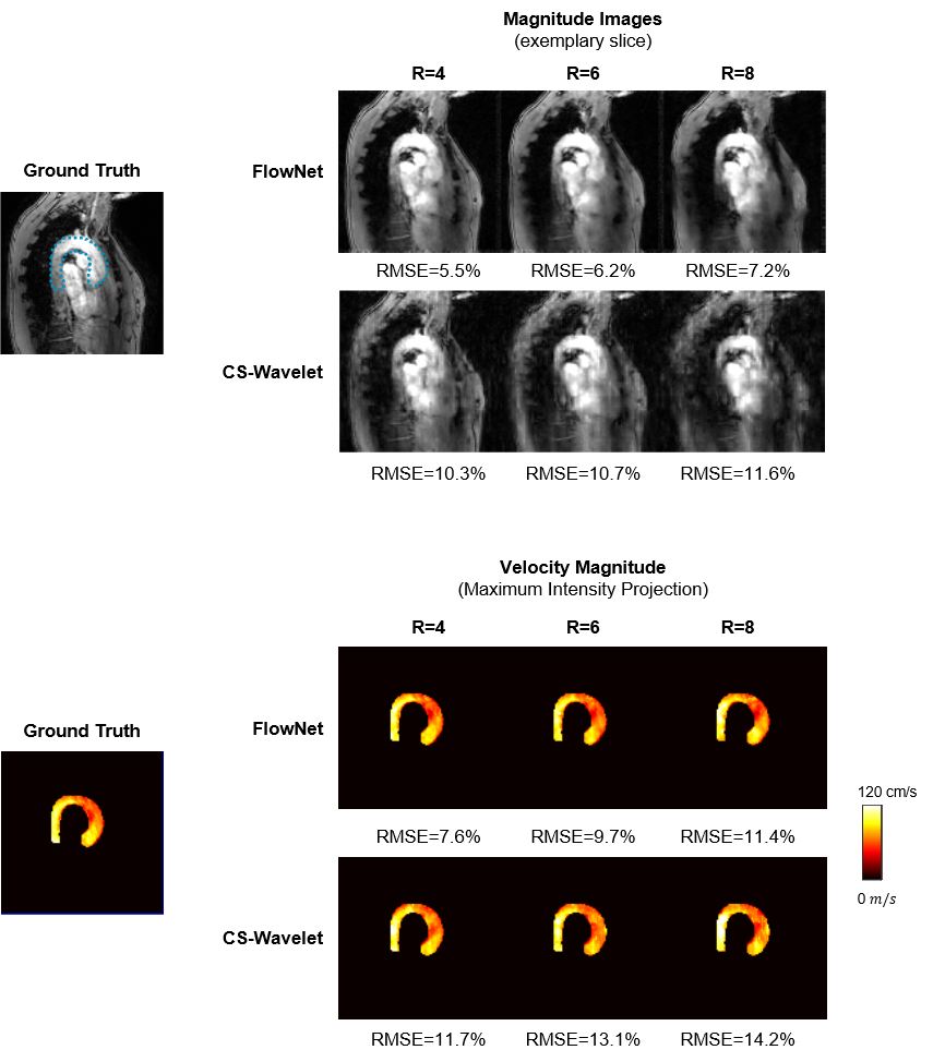
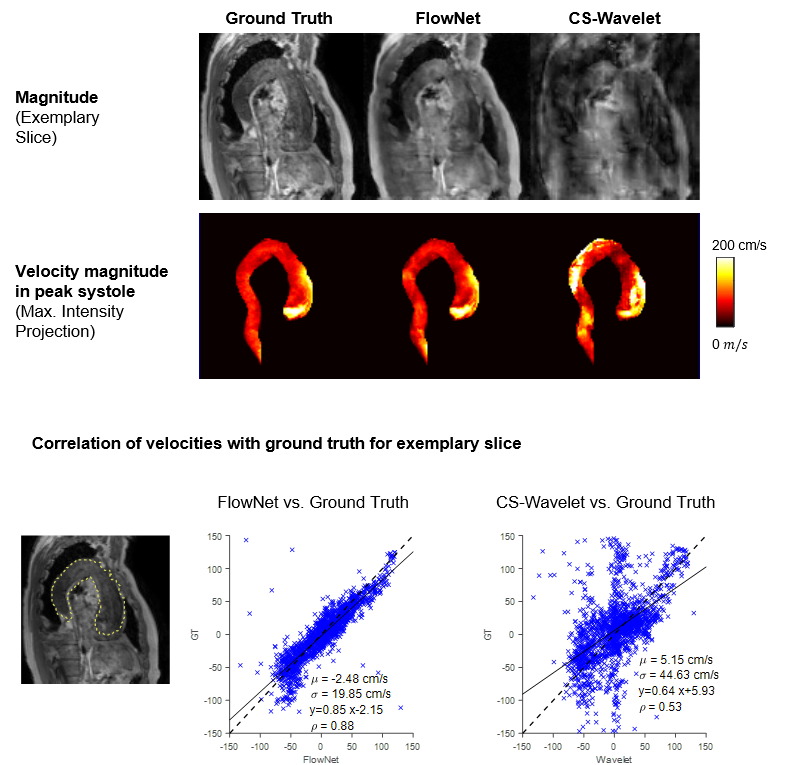
Reconstruction results for different acceleration factors are compared in Figure 2. FlowNet consistently outperforms CS-Wavelet in terms of RMSE of magnitude and velocity magnitude. Figure 3 shows reconstruction results for the retrospectively undersampled patient dataset. FlowNet accurately depicts the flow field whereas CS-Wavelet shows artifacts and cannot preserve the jet at the inbound section of the aorta.

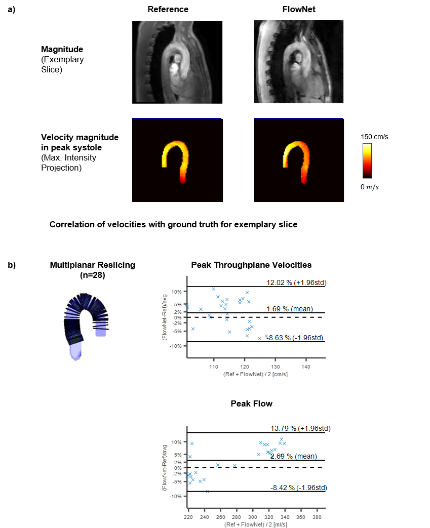
Reconstruction results for prospectively undersampled data are shown in Figure 4. Assessment of peak velocities and peak flow show good agreement with the reference measurement.

Discussion

Conclusion

Acknowledgements

References

1. Lustig M, Donoho D, Pauly JM. Sparse MRI: The application of compressed sensing for rapid MR imaging. Magnetic Resonance in Medicine. 2007;58(6):1182–1195.

2. Sodickson DK, Otazo R, Candes E. Low-rank plus sparse matrix decomposition for accelerated dynamic MRI with separation of background and dynamic components. 2015;1136:1125–1136.

3. Valvano G, Martini N, Huber A, Santelli C, Binter C, Chiappino D, Landini L, Kozerke S. Accelerating 4d flow MRI by exploiting low-rank matrix structure and hadamard sparsity. Magnetic resonance in medicine. 2017;78(4):1330–1341.

4. Feng L, Axel L, Chandarana H, Block KT, Sodickson DK, Otazo R. XD-GRASP: Golden-angle radial MRI with reconstruction of extra motion-state dimensions using compressed sensing. Magnetic resonance in medicine. 2016;75(2):775–788.

5. Rich A, Potter LC, Jin N, Ash J, Simonetti OP, Ahmad R. A Bayesian model for highly accelerated phase-contrast MRI. Magnetic Resonance in Medicine. 2016;76(2):689–701.

6. Hammernik K, Klatzer T, Kobler E, Recht MP, Sodickson DK, Pock T, Knoll F. Learning a variational network for reconstruction of accelerated MRI data. Magnetic Resonance in Medicine. 2018;79(6):3055–3071.

7. Vishnevskiy V, Sanabria SJ, Goksel O. Image Reconstruction via Variational Network for Real-Time Hand-Held Sound-Speed Imaging. In: International Workshop on Machine Learning for Medical Image Reconstruction. 2018. p. 120–128.

8. Kingma DP, Ba J. Adam: A method for stochastic optimization. arXiv preprint arXiv:1412.6980. 2014.

9. Pruessmann KP, Weiger M, Scheidegger MB, Boesiger P. SENSE: Sensitivity encoding for fast MRI. Magnetic Resonance in Medicine. 1999;42(5):952–962.

10. Jonas Walheim and Sebastian Kozerke. 5D Flow MRI – Respiratory Motion Resolved Accelerated 4D Flow Imaging Using Low-Rank + Sparse Reconstruction. In: Proceedings of the 26th Annual Meeting of ISMRM. Presented at the ISMRM. 2018. p. 0032.

11. Zhang T, Pauly JM, Vasanawala SS, Lustig M. Coil compression for accelerated imaging with Cartesian sampling. Magnetic Resonance in Medicine. 2013;69(2):571–582.

12. Roemer PB, Edelstein WA, Hayes CE, Souza SP, Mueller OM. The NMR phased array. Magnetic Resonance in Medicine. 1990;16(2):192–225.