4649
Semi-Supervised Learning for Reconstructing Under-Sampled MR Scans1Electrical Engineering, Stanford University, Stanford, CA, United States, 2Radiology, Stanford University, Stanford, CA, United States
Synopsis
Supervised deep-learning approaches have been applied to MRI reconstruction, and these approaches were demonstrated to significantly improve the speed of reconstruction by parallelizing the computation and using a pre-trained neural network model. However, for many applications, ground-truth images are difficult or impossible to acquire. In this study, we propose a semi-supervised deep-learning method, which enables us to train a deep neural network for MR reconstruction without using fully-sampled images.
Target audience
MR scientists working on MRI reconstruction.Purpose
Accelerating MRI by under-sampling in the spatial-frequency domain (k-space) is commonly used to reduce motion-related artifacts and improve scan efficiency. Parallel imaging and compressed sensing (PICS) has been widely used to reconstruct under-sampled MR scans[1]. However, these techniques may be computationally expensive for high spatial/temporal resolution acquisitions, resulting in significant delays in patient care. Recently, supervised deep learning approaches have been applied to MRI reconstruction, and these approaches have been demonstrated to significantly improve the speed of reconstruction by parallelizing the computation and using a pre-trained neural network model[2-5]. In these methods, it is necessary to collect sufficient ground-truth images to train the neural network. However, for many applications, such as dynamic contrast enhancement, perfusion, or multi-dimensional high resolution acquisitions, ground-truth images are difficult or impossible to acquire[6]. To enable deep-learning reconstruction of MRI in these settings, we propose a semi-supervised deep-learning method, which enables us to train a deep neural network for MR reconstruction without fully-sampled images.Method
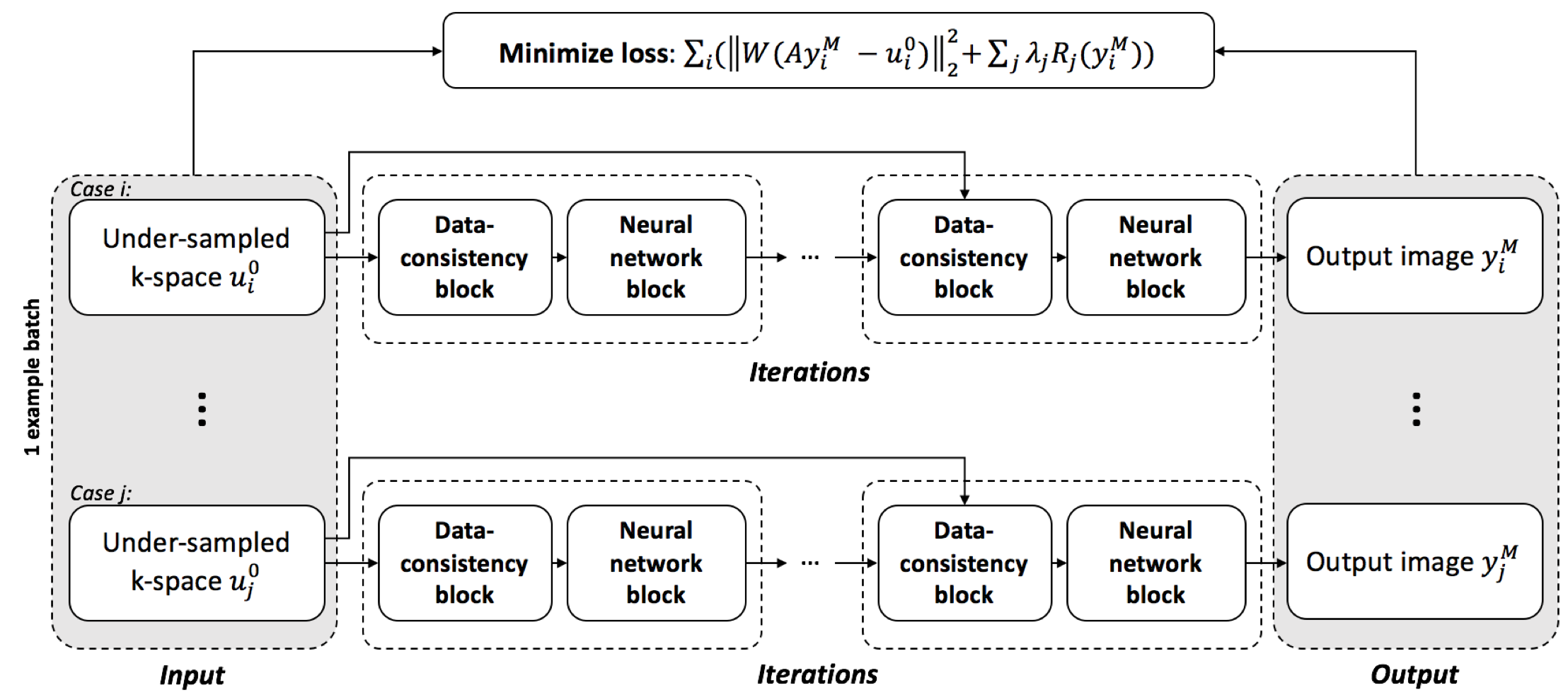
The proposed method is illustrated in Fig. 1. Batches of under-sampled k-space measurements were randomly chosen as the input to the network. The network contains four recurrences of data-consistency blocks and neural-network blocks. A loss function containing a data-consistency term and a regularization term was minimized with backpropagation during the training:$$loss=\Sigma_i(||W(Ay^M_i-u^0_i)||^2_2 + \Sigma_j \lambda_j R_j(y^M_i))$$
where $$$y^M_i$$$ is the output image of the entire network for the $$$i^{\text{th}}$$$ slice, $$$u^0_i$$$ is the under-sampled k-space measurements of the $$$i^{\text{th}}$$$ slice, $$$W$$$ denotes an optional window function, and $$$A$$$ denotes the encoding operator from image to k-space, which includes coil sensitivity maps when the data is acquired with multiple coil channels. $$$||W(Ay^M_i-u^0_i)||^2_2$$$ denotes the data consistency term, and $$$\Sigma_j \lambda_j R_j(y^M_i))$$$ denotes regularization terms. In this study, we use total variation and wavelet transforms as the regularization terms. Since this loss function only depends on the under-sampled measurements and the output of the network, the training process requires no fully-sampled images.
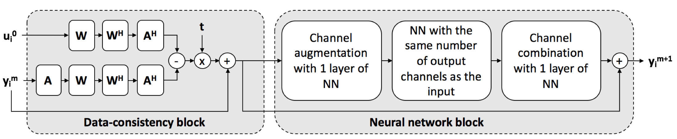
The network architecture of one step of data consistency and neural network blocks is shown in Fig. 2. The data-consistency block implements an iterative shrinkage thresholding algorithm (ISTA)[7]. It uses k-space measurements $$$u^0_i$$$ of the $$$i^{\text{th}}$$$ slice and the output of previous neural network block $$$y^M_i$$$ as inputs. The neural network block implements a residual neural network (ResNet)[8], which contains a channel augmentation layer, 3 convolutional layers with 12 features and a kernel size of 9x9, and a channel combination layer.
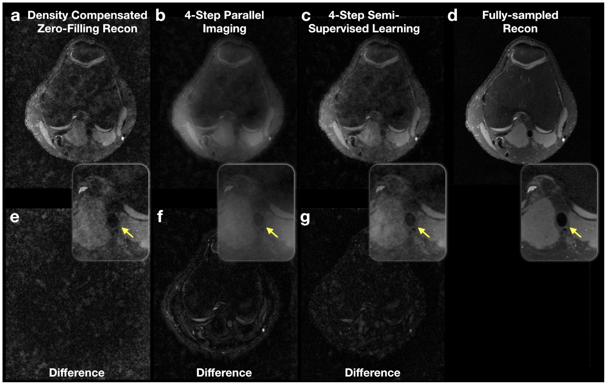
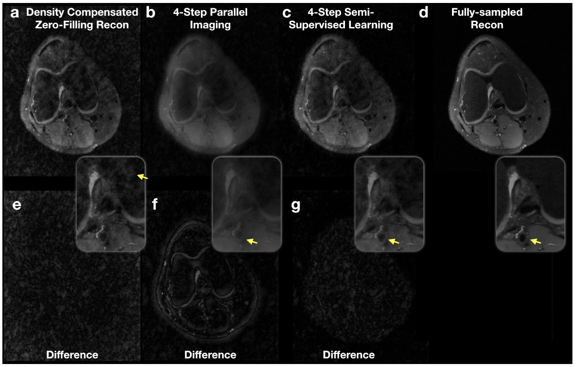
In the training stage, k-spaces from fifteen fully-sampled 3D FSE scans (3840 samples in total, available on http://mridata.org/) were down-sampled with randomly generated uniform sampling patterns (but each includes a 10x10 fully-sampled center) at a total under-sampling factor of 6.25. Training was performed with a batch size of 8. The entire training pipeline was implemented in Tensorflow and performed on an NVIDIA GTX 1080Ti GPU. To evaluate the proposed semi-supervised learning approach, we compared the output images of the trained network with the PICS reconstruction under the same four ISTA iterations. Normalized root-mean squared error (RMSE) was computed between the reconstructed images and fully-sampled images.
Results
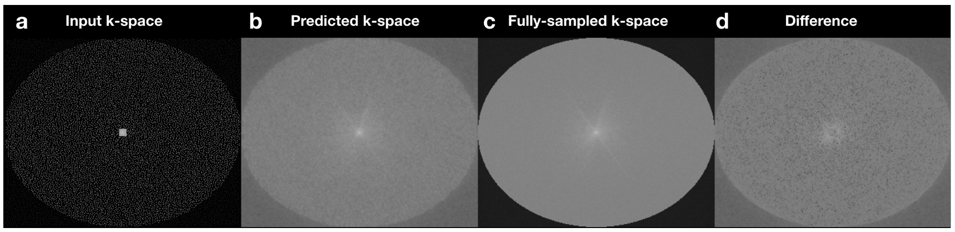
With the same number of ISTA iterations, the proposed CNN approach improved the image quality over conventional parallel imaging reconstruction at an under-sampling factor of 6.25 (Fig. 3-4). The CNN approach also reduced the aliasing artifacts caused by under-sampling, in comparison with density-compensated zero-filling reconstructions (Fig. 3-4). Images reconstructed with the trained CNN yielded a normalized RMSE of 3.6±0.24% while parallel imaging achieved 4.1±0.13% RMSE with the same number of ISTA iterations. The proposed method was able to fill in missing samples in the k-space; however, the under-sampling pattern was still visible in the predicted k-space (Fig. 5).Discussion and Conclusion
This work introduces a semi-supervised deep-learning approach to MRI reconstruction by training a deep neural network with a loss function that enforces both data consistency and additional image features. Compared to conventional methods, the proposed approach can train a deep neural network without fully-sampled images and improve the image quality of parallel imaging under the same number of ISTA iterations. This enables deep learning reconstruction when fully-sampled k-spaces are difficult or impossible to acquire. Exploring and evaluating the performance of different loss functions, regularization terms, and sampling patterns will be our future work.Acknowledgements
NIH/NIBIB R01 EB009690, R01 EB019241, and GE Healthcare.References
1. Lustig M, et al. Sparse MRI: The application of compressed sensing for rapid MR imaging. Magnetic resonance in medicine. 2007, 58(6):1182-1195.
2. Hammernik K, et al. Learning a Variational Network for Reconstruction of Accelerated MRI Data. arXiv: 1704.00447 [cs.CV] (2017).
3. Yang Y, et al. ADMM-Net: A Deep Learning Approach for Compressive Sensing MRI. Nips 10–18 (2017).
4. Diamond S, et al Unrolled Optimization with Deep Priors. arXiv: 1705.08041 [cs.CV] (2017).
5. Jin KH, et al. Deep Convolutional Neural Network for Inverse Problems in Imaging. arXiv: 1611.03679 [cs.CV] (2016).
6. Zhang T, et al. Fast pediatric 3D free-breathing abdominal dynamic contrast enhanced MRI with high spatiotemporal resolution. J. Magn. Reson. Imaging 41, 460–473 (2015).
7. Beck A, et al. A fast iterative shrinkage-thresholding algorithm for linear inverse problems. SIAM journal on imaging sciences. 2009 Mar 4;2(1):183-202.
8. He K, et al. Deep residual learning for image recognition. In Proceedings of The IEEE conference on computer vision and pattern recognition 2016 (pp. 770-778).
Figures