4648
Unpaired Super-Resolution GANs for MR Image Reconstruction1Electrical Engineering, Stanford University, Stanford, CA, United States, 2Radiology, Stanford University, Stanford, CA, United States
Synopsis
While undersampled MRI data is easy to obtain, lack of high-quality labels for dynamic organs impedes the common supervised training of deep neural nets for MRI reconstruction. We propose an unpaired training super-resolution model with pure GAN loss to use a minimal amount of labels but all available low-quality data for training. Leveraging Wasserstein-GANs with gradient penalty followed by a data-consistency refinement high-quality Knee MR images are recovered from 3-fold undersampled single coil measurements using 20% of the labels compared with a paired training model.
Introduction
Reconstructing high-quality magnetic resonance images (MRIs) is compute-intensive with conventional compressed sensing (CS) analytics1 -- image quality has to be sacrificed for real-time imaging. Existing work2 using neural networks for MRI reconstruction runs at the order of hundred times faster than CS-MRI schemes. However, lack of high-quality MR images (labels) for dynamic organs impedes the prevailing supervised training of deep nets for reconstruction. This fact motivates our unpaired training approach. Our approach does not require one-to-one (i.e. paired) supervision thus allows using different number of high- and low- quality data for training. MRI recovery typically solves a linear inverse system $$$\mathbf{y}=\mathbf{\Phi x}$$$ to find $$$\mathbf{x} \in \mathbb{C}^n$$$ from partial frequency domain samples $$$\mathbf{y} \in \mathbb{C}^m$$$ ($$$m \ll n$$$). Our model is trained to invert the map so that for test data $$$\mathbf{y}$$$ we can automatically recover its corresponding $$$\mathbf{x}$$$ as $$$f(\mathbf{y})$$$ for a neural network $$$f$$$. Several works2,3,4 uses generative adversarial networks (GANs) for MRI reconstruction; all of them use pixel-wise losses and some perceptual losses thus require paired input and label. The paired losses are essential to the performance of super-resolution tasks 5; authors in [2] point out that their pixel-wise $$$\ell_1$$$ cost is responsible of attenuating noise in the generated images. In the paired approach, a corresponding $$$\mathbf{x}$$$ is given for each $$$\mathbf{y}$$$ during training. We consider a more practical case where a set of noisy observations $$$\mathcal{Y}:=\{\mathbf{y}_i\}^M_{i=1}$$$ are relatively easy to obtain, and the acquisition of a set of high-quality samples $$$\mathcal{X}:=\{\mathbf{x}_j\}^N_{j=1}$$$ is expensive ($$$N\ll M$$$), thus pairing between $$$\mathbf{x}$$$ and $$$\mathbf{y}$$$ cannot exist. We aim to use a minimal $$$N$$$ for training.Methods
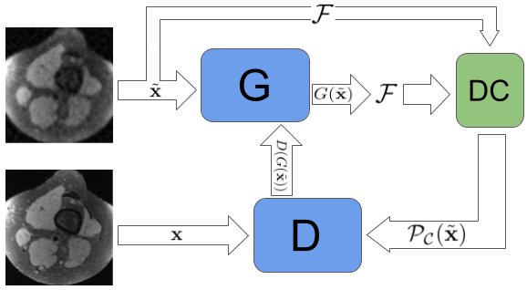
We propose using GANs to learn and approximate the distribution of high-quality MRIs. During training, the input to the generator (G) is $$$\tilde{\mathbf{x}}=\mathcal{F}^{-1}(\mathbf{y})$$$, where $$$\mathcal{F}$$$ represents two-dimensional discrete Fourier transform (DFT), and the noisy observation $$$\mathbf{y}$$$ zero pads missing frequencies according to the sampling mask $$$\Omega$$$. The G is responsible for reconstructing $$$\tilde{\mathbf{x}}$$$ mimicking the distribution of $$$\mathbf{x}$$$. Training of WGANs6 is derived to minimize the Wasserstein-1 distance between the underlying ground-truth data distribution and the distribution implicitly defined by the outputs of the G. The discriminator (D) aims to assign a confidence value to each of its input, which is low on generated data and high on real data. The learning objectives for G and D are:
$$ \min_{\Theta_g,\Theta_d}L_D(\Theta_d)=\mathbb{E}\big[D(\mathcal{P}_{\mathcal{C}}(\tilde{\mathbf{x}});\Theta_g);\Theta_d)\big] - \mathbb{E}\big[D(\mathbf{x};\Theta_d)\big] + \eta \mathbb{E}_{\hat{\mathbf{x}} \sim P}\big[(|| \nabla_{\hat{\mathbf{x}}} D(\hat{\mathbf{x}};\Theta_d)||_2 - 1)^2 \big]$$$$\min_{\Theta_g,\Theta_d} L_G(\Theta_g)= -\mathbb{E}\big[D(\mathcal{P}_{\mathcal{C}}(\tilde{\mathbf{x}});\Theta_g);\Theta_d)\big] $$
where $$$\Theta_g, \Theta_d$$$, denoting parameters for G and D respectively, are updated in an alternating fashion based on stochastic gradient descent. The last term in $$$L_D(\Theta_d)$$$ is the gradient penalty (GP) advocated in WGAN-GP7 to enforce the discriminator function to lie in the space of 1-Lipschitz functions, where $$$\eta$$$ is a constant coefficient. $$$\hat{\mathbf{x}}$$$ is sampled uniformly from a distribution $$$P$$$, which is induced by straight lines between pairs of points sampled from the ground-truth data distribution and the G output's distribution. We use a data-consistency (DC) layer after G, which is crucial to stabilizing the training of G when no pixel-wise supervision is present. Equation below defines the DC layer output $$$\mathcal{P}_{\mathcal{C}}(\tilde{\mathbf{x}})$$$, where $$$G(\tilde{\mathbf{x}})$$$ is the output of G: $$\mathcal{P}_{\mathcal{C}}(\tilde{\mathbf{x}})=\mathcal{F}^{-1}\{\Omega\odot\mathcal{F}\{\tilde{\mathbf{x}}\}+(1-\Omega)\odot\mathcal{F}\{G(\tilde{\mathbf{x}})\}\}.$$ Fig.1 illustrates the training procedure of our model.
Results
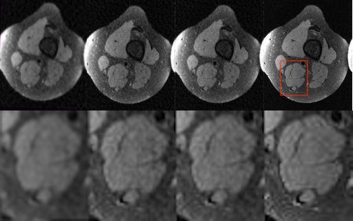
The G is a deep residual network (ResNet)8 with four residual blocks followed by $$$3$$$ conv layers. The discriminator (D) consists of 7 conv layers with Leaky ReLU activation9. We use Adam10 with a learning rate of $$$5\times 10^{-4}$$$ for optimization and $$$\eta=10$$$. We examine our model on a Knee dataset where there are high-quality MRI scans for 19 patients with 3D volumes of size $$$320 \times 160 \times 128$$$ (in total 6,080 2D images). The low-quality data is obtained by applying an $$$n$$$-fold mask in the frequency domain on the high-quality data. Our training set contains scans from 17 patients and our test set contains scans from 2 patients. We train our model using high-quality volumes from 3 and 6 patients, and low-quality volumes from all 17 patients in the training set. To examine effectiveness of using the unpaired approach and more low-quality inputs, we trained the GANCS2 model with 95% pixel-wise loss on the low- and high-quality pairs from 3 patients -- the resulting images are clearly unacceptable. We tried recovering inputs undersampled by 3-, 4- and 5-fold masks. The result from 3-fold undersampled inputs, demonstrated by Fig. 2 and 3, is of high diagnostic quality, the result from 4-fold undersampled inputs is arguably acceptable, the result from 5-fold undersampled inputs is too noisy to provide accurate details (see also Fig. 4). We conclude that with unpaired pure GAN training, our model is limited to recovering maximum 3-4 fold undersampled MRIs.Acknowledgements
Authors are grateful for support of the NIH (R01EB009690, R01EB026136) and GE Healthcare.References
- Michael Lustig, David Donoho, and John M Pauly. Sparse mri: The application of compressed sensing for rapid MR imaging. Magnetic Resonance in Medicine: An Official Journal of the International Society for Magnetic Resonance in Medicine, 58(6):1182–1195, 2007.
- M. Mardani, E. Gong, J. Y. Cheng, S. S. Vasanawala, G. Zaharchuk, L. Xing, and J. M. Pauly. Deep generative adversarial neural networks for compressive sensing (GANCS) MRI. IEEE Transactions on Medical Imaging, pages 1–1, 2018.
- Tran Minh Quan, Thanh Nguyen-Duc, and Won-Ki Jeong. Compressed sensing MRI reconstruction using a generative adversarial network with a cyclic loss. IEEE transactions on medical imaging, 37(6):1488–1497, 2018.
- Guang Yang, Simiao Yu, Hao Dong, Greg G. Slabaugh, Pier Luigi Dragotti, Xujiong Ye, Fangde Liu, Simon R. Arridge, Jennifer Keegan, Yike Guo, and David N. Firmin. Dagan: Deep de-aliasing generative adversarial networks for fast compressed sensing MRI reconstruction. IEEE Transactions on Medical Imaging, 37:1310–1321, 2018.
- C. Ledig, L. Theis, F. Huszár, J. Caballero, A. Cunningham, A. Acosta, A. Aitken, A. Tejani, J. Totz, Z. Wang, and W. Shi. Photo-realistic single image super-resolution using a generative adversarial network. In 2017 IEEE Conference on Computer Vision and Pattern Recognition (CVPR), pages 105–114, July 2017.
- K. He, X. Zhang, S. Ren, and J. Sun. Deep residual learning for image recognition. In 2016 IEEE Conference on Computer Vision and Pattern Recognition (CVPR), pages 770–778, June 2016.
- Ishaan Gulrajani, Faruk Ahmed, Martin Arjovsky, Vincent Dumoulin, and Aaron C Courville. Improved training of wasserstein GANs. In Advances in Neural Information Processing Systems, pages 5769–5779, 2017.
- Martin Arjovsky, Soumith Chintala, and Léon Bottou. Wasserstein generative adversarial networks. In Doina Precup and Yee Whye Teh, editors, Proceedings of the 34th International Conference on Machine Learning, volume 70 of Proceedings of Machine Learning Research, pages 214–223, International Convention Centre, Sydney, Australia, 06–11 Aug 2017. PMLR.
- Andrew L Maas, Awni Y Hannun, and Andrew Y Ng. Rectifier nonlinearities improve neural network acoustic models. In Proc. icml, volume 30, page 3, 2013.
- Diederik P. Kingma and Jimmy Ba. Adam: A method for stochastic optimization. CoRR, abs/1412.6980, 2014.
- Zhou Wang, A. C. Bovik, H. R. Sheikh, and E. P. Simoncelli. Image quality assessment: from error visibility to structural similarity. IEEE Transactions on Image Processing, 13(4):600–612, April 2004.
Figures