Synopsis

For multi-dimensional RF pulses, neural networks and deep learning may boost the clinical applicability by allowing very rapid pulse predictions, based on offline training and offline generated training libraries. This can potentially offer opportunities, for example, to revive slow, abandoned pulse design techniques, or to include many more constraints or complexities into the pulse designs that until now were infeasible to bring into a clinical setting, since the neural network will simply learn the features of the training library. We are demonstrating the principle with numerical simulations, and phantom and in vivo experiments.

Purpose

To introduce a novel multi-dimensional RF pulse design technique based on neural networks (NN) and deep learning (DL), thereby improving the workflow and applicability of acquisitions with multi-dimensional RF pulses.

Methods

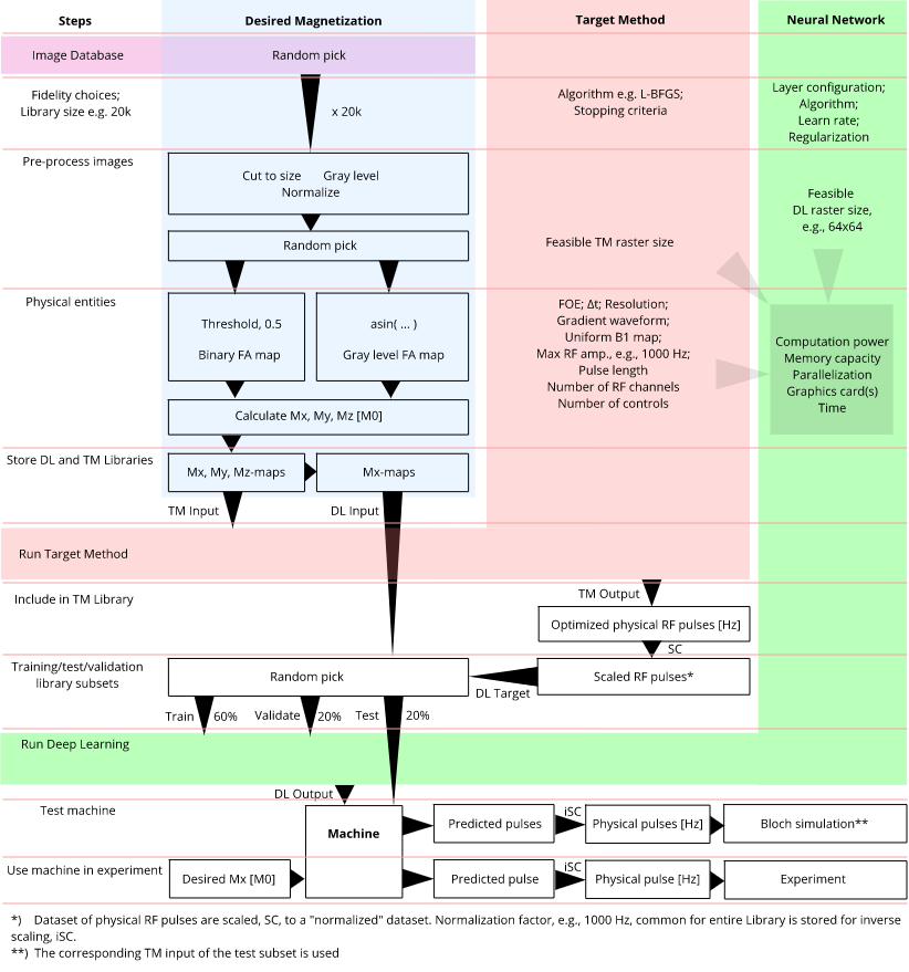
Figure 1 shows the workflow of the proposed method.

Training library: Imagenet [1] images were randomly picked and cut to 64-by-64 pixels, grey scaled, and normalized. Random black-white (BW) 2D target magnetizations were generated by thresholding the images, while grey scale images (Gr) were used for variable flip angle target patterns. Image level values were converted to flip angles by $$$\sin^{-1}(\mathrm{value})$$$, i.e., $$$\leq 90^\circ$$$ flips. Input data (target magnetizations) were fed to an optimal control RF pulse design target method (TM) [2]. The pulses were conformed to a 6.39-ms spiral k-space trajectory [3], 10-µs dwell time, and a 1-kHz maximum RF limit. Optimized pulses (output data) were obtained on a computer cluster using MATLAB 2016a (Mathworks, Natick). The input and output data constituted the input and (supervision) target data for the neural network, respectively. We produced a total 20k BW and 20k Gr examples. We assessed the question of feasible library sizes by splitting a 20k-BW library into smaller subsets (1k, 2k, 3k, 4k, 5k, 7.5k, 10k, 12.5k, 15k), and trained NNs for each of those as well as the 20k library.

Neural network: The NN structure consisted of the following layers: (1) 64-by-64-by-1 image input, (2) 4096-by-1 fully connected, (3) rectified linear unit, (4) 3000-by-1 fully connected, (5) rectified linear unit, (6) 1278-by-1 fully connected, and (7) 1278-by-1 regression. The size 1278 corresponds to 2x639, which is the number of RF controls (x- and y-channels).

Deep learning: The Neural Network toolbox from MATLAB 2018a was used for DL on a workstation with two Intel Xeon Gold 2.2 GHz processors with 28 cores in total, 512 GB RAM and an NVIDIA Tesla P100 16GB GPU. The Stochastic Gradient Descent with Momentum (SGDM) algorithm was used for training the NNs (1000 epochs). We split the training libraries into training/validating/testing ratios of 0.6/0.2/0.2. Training with validation of the larger libraries took around 24 hours.

Simulations: Magnetization simulations were conducted with the Bloch simulator of Ref. [4]. We considered only the $$$M_x$$$-component in error evaluations, i.e., the normalized root mean square error (NRMSE).

Experiments: Phantom and in vivo experiments were conducted on a Siemens 3T PrismaFit (Erlangen, Germany). The RF pulses (NN-predicted and TM-calculated) were implemented into a 2D RF spin echo sequence (TE 20 ms, TR 1 s, NA 2, FOV 25 cm) designed with Pulseq [5].

Results and Discussion

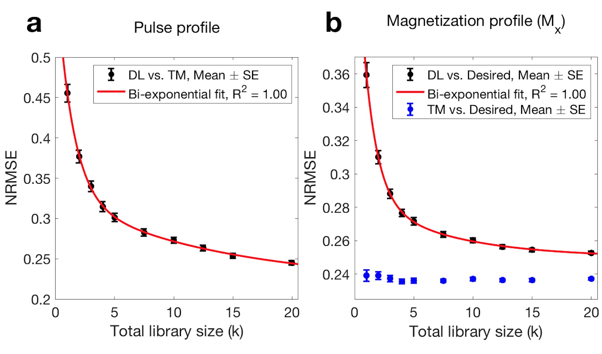
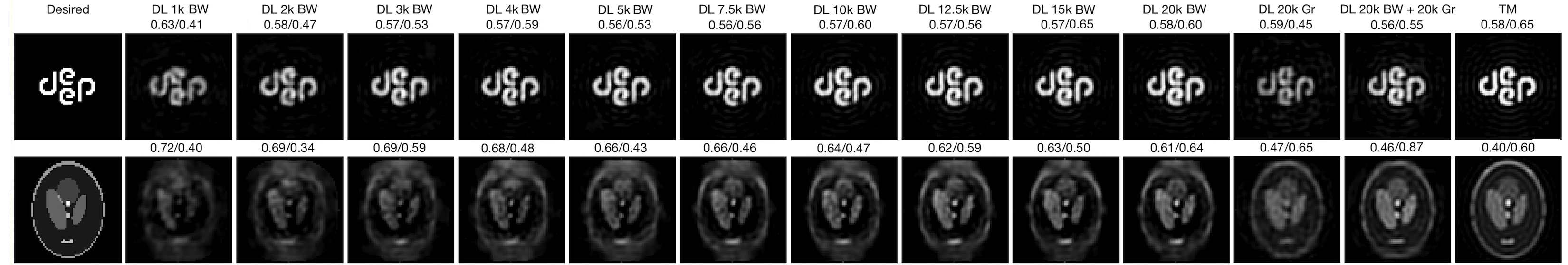
The library size assessment results are shown in Figure 2 with NRMSE values of the test data shown as L-curves of mean values and standard error bars. We show both the NRMSEs of DL-predicted pulses against the TM-calculated pulses (Fig. 2a), and the corresponding magnetization profile simulations against the target profiles (Fig. 2b). Numerical examples from these trained NNs are shown simulated in Figure 3, also showing results of the NN trained with only Gr-type inputs, and a NN trained with BW- and Gr-types together.

The NNs did not include RF constraints, but rely on the TM. Relative peak RF amplitudes for DL-predicted pulses were on average within the 1-kHz limit. With the current form of the NN, we propose to use VERSE [6], clipping, or TM-limit regularization to overcome/ minimize occasional RF overshoots, for example. For the simulations and experiments, our test cases did not require better RF control.

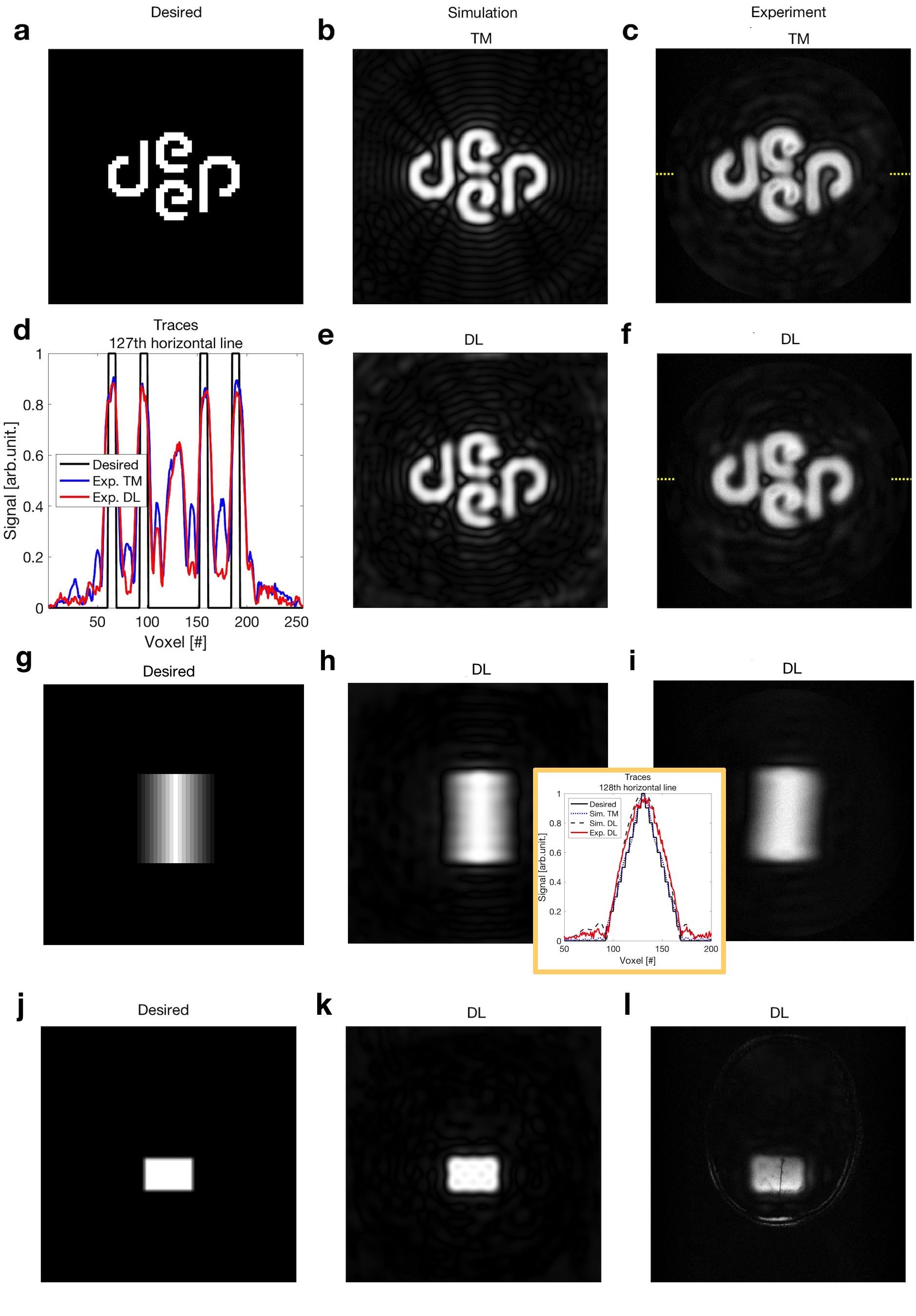
Experimental data are shown in Figure 4, together with numerical simulations. We used a 10k-BW library for experiments, but also show by example how a Gr-type target can be employed as well Fig. 4g-i.

The 2D RF pulse prediction time was on average 7 ms on commodity hardware.

Conclusion

Acknowledgements

References

1. Deng J, Dong W, Socher R, Li L-J, Li K, Fei-Fei L. ImageNet: A Large-Scale Hierarchical Image Database. In: CVPR09; 2009.

2. Vinding MS, Guérin B, Vosegaard T, Nielsen NC. Local SAR, global SAR, and power-constrained large-flip-angle pulses with optimal control and virtual observation points. Magn. Reson. Med. 2017;77:374–384

3. Lustig M, Kim S-J, Pauly JM. A fast method for designing time-optimal gradient waveforms for arbitrary k-space trajectories. IEEE Transactions on Medical Imaging 2008;27:866–873

4. Vinding MS, Brenner D, Tse DHY, et al. Application of the limited-memory quasi-Newton algorithm for multi-dimensional, large flip-angle RF pulses at 7T. Magnetic Resonance Materials in Physics, Biology and Medicine 2017;30:29–39

5. Layton KJ, Kroboth S, Jia F, et al. Pulseq: A rapid and hardware-independent pulse sequence prototyping framework: Rapid Hardware-Independent Pulse Sequence Prototyping. Magnetic Resonance in Medicine 2017;77:1544–1552

6. Conolly S, Nishimura D, Macovski A, Glover G. Variable-rate selective excitation. Journal of Magnetic Resonance (1969) 1988;78:440–458