Synopsis

Optimal control (OC) methods for RF pulse design are useful in cases where the small-tip angle (STA) approximation is violated. Furthermore, designs with physically meaningful constraints (e.g., RF peak amplitude and integrated power) eliminate the need for parameter tuning to create realizable pulses. In this abstract we introduce a constrained fast OC method that easily generalizes to a variety of RF pulse designs. We demonstrate with examples of SMS and spectral prewinding pulses in simulation and in vivo. The constrained fast OC method guarantees that RF pulses will meet physical constraints while outperforming their non-OC counterparts.

Introduction

RF pulse design is classically a regularized weighted least-squares optimization problem¹ under the small-tip angle (STA) approximation². Recently, constrained pulse design^3-5 has become popular for designing physically realizable pulses without “check-and-redesign” parameter tuning.

Meanwhile, optimal control (OC) approaches have enabled the design of large-tip angle (LTA) pulses^6-7. In this work we design constrained RF pulses via the fast OC method⁷ that is simple and computationally inexpensive, but previous fast OC design methods did not include explicit constraints on RF amplitude and integrated power.

Methods

The general pulse design problem we solve here is

$$\widehat{\textbf{b}}=\mathrm{argmin}_{\textbf{b}}=\vert\vert\;\mathrm{Bloch}(\textbf{b})-\textbf{d}\vert\vert_{\textbf{W}}^{2}$$

$$\mathrm{s.t.}\;\;\mathrm{RF}\;\;\mathrm{constraints}$$

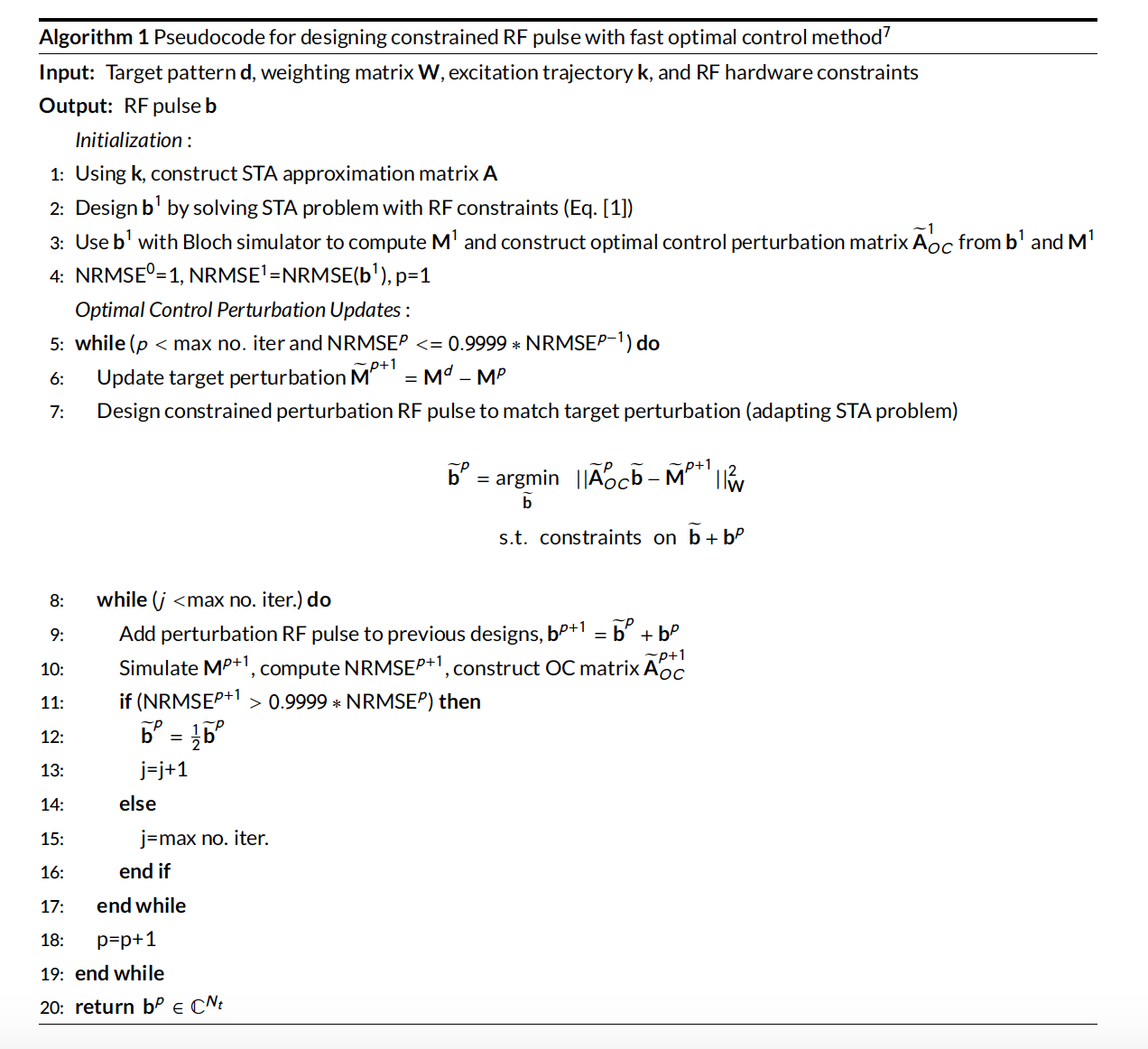
with RF pulse b, target pattern d, and weighting matrix W. For LTA pulses, we linearize the Bloch equation with OC via perturbation updates⁷ enforcing RF constraints directly at each update. This is unlike the STA approximation², in which the Bloch equation evaluation of b is substituted with the linear STA matrix A. Figure 1 provides the pseudocode for this process. Importantly, the inner constrained problem is linear and can be solved with a variety of readily available methods (e.g., FISTA, CVX, etc.). The only values the user must provide the algorithm are the maximum number of iterations and % change in normalized root mean-squared error (NRMSE) for stopping criteria.

We designed two distinct RF pulse types to demonstrate the flexibility of this constrained fast OC approach. First, we designed a 90° simultaneous multislice (SMS) pulse with multiband factor MB=3 and compared to the standard implementation of phase shifted and summed slice-selective pulses, here Shinnar Le-Roux (SLR) pulses⁸. The SLR SMS pulse was designed with a time bandwidth product of 4, default SLR filter parameters, and a pulse length of 2.736 ms chosen to exactly meet peak RF amplitude constraints (0.2 G) after optimal phase modulation for peak amplitude reduction⁹. The constrained SMS MB=3 pulse was designed to have the same pulse length with constraints on peak amplitude and integrated RF power also matching the SLR SMS pulse.

Next, we designed a spectral prewinding slab-selective pulse pair¹⁰ and obtained in vivo human brain results using the small-tip fast recovery (STFR) sequence¹¹ (FA/TE/TR=3.5°/3.82 ms/14.836 ms). Despite the small target flip angle, we previously found that prewinding pulses can exceed STA at intermediate pulse time points, making the OC approach useful. The STFR pulse pair was designed with a peak amplitude constraint of 0.2 G and the constrained OC pulses were compared to constrained pulses designed only using the STA approximation.

Results

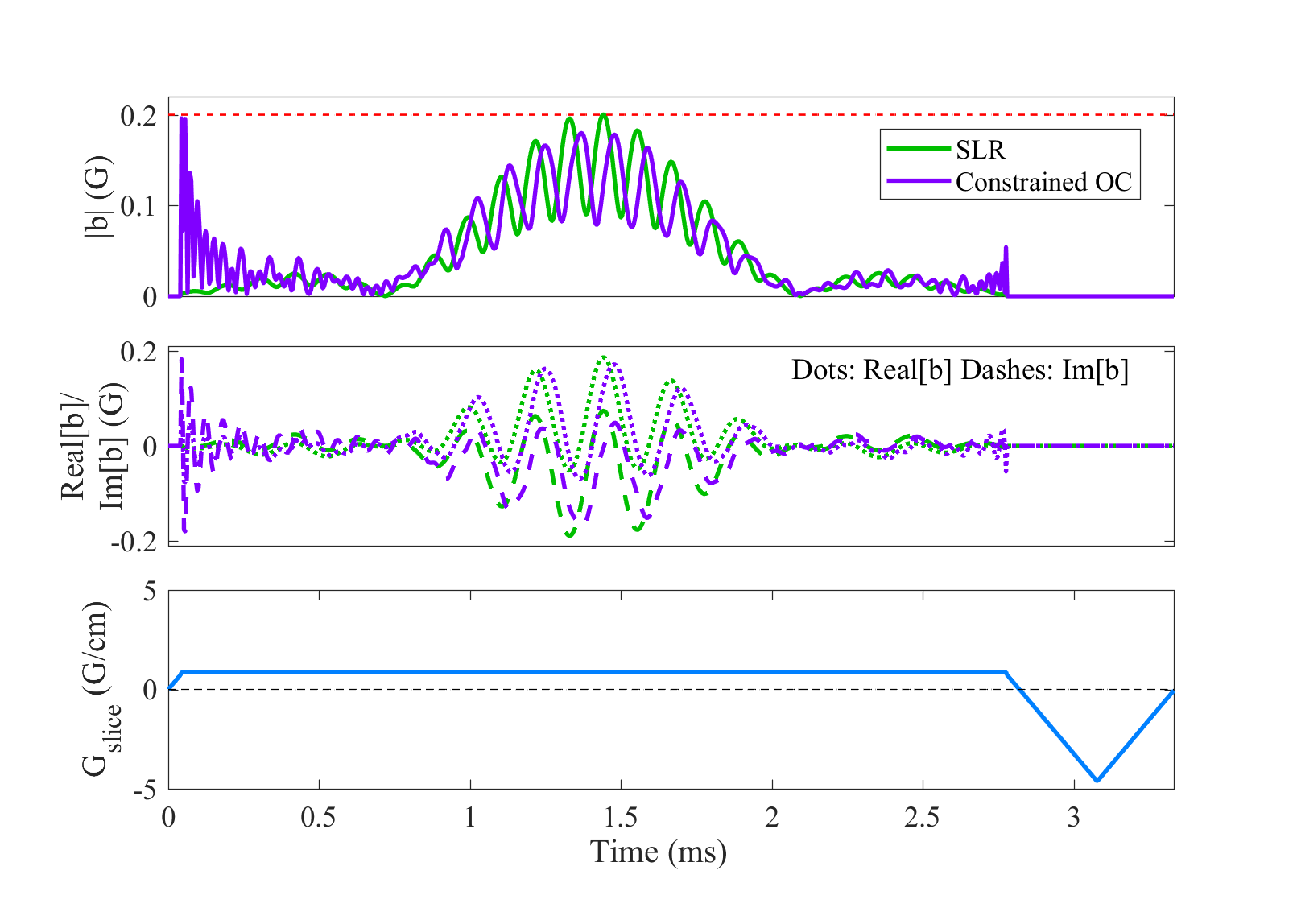
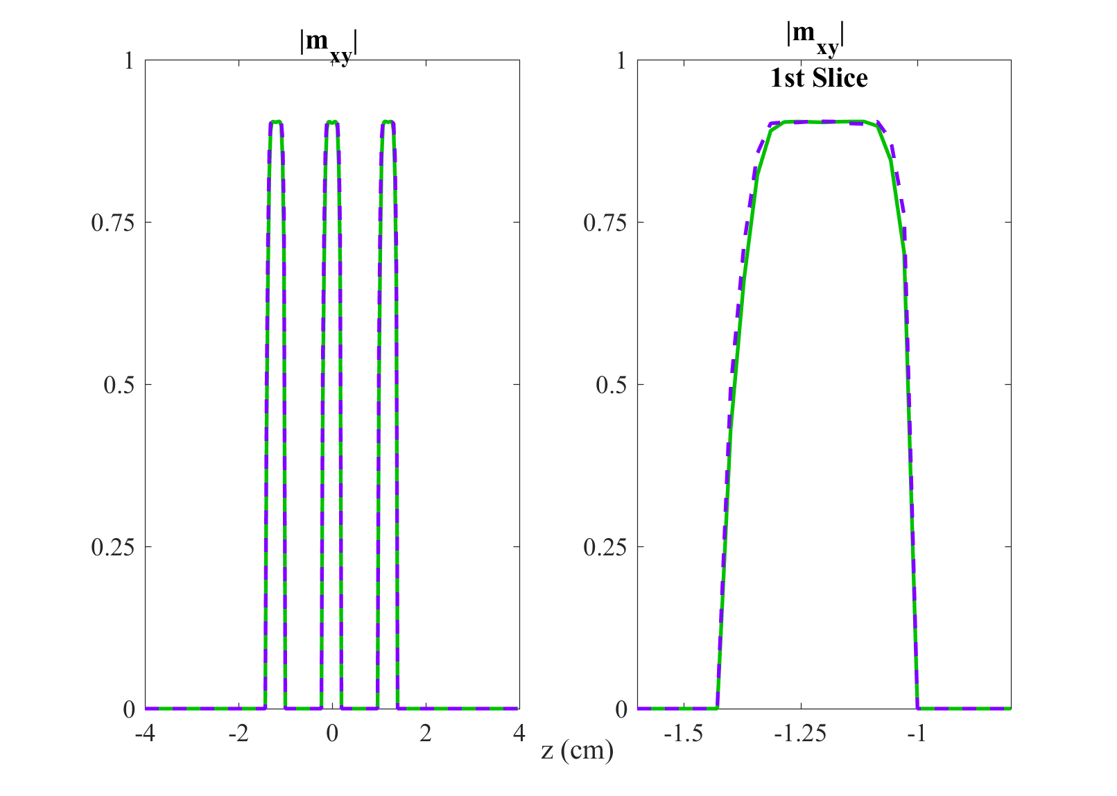
Figure 2 shows the RF and slice-select gradient waveforms for the SMS MB=3 pulses designed with the SLR method and the proposed constrained OC method. Figure 3 shows the simulated magnetization magnitude and slice profiles at TE for both pulses. Compared to a target magnetization of 90° MB=3 slices, the magnitude NRMSE is 0.10 for the SLR pulse pair and also 0.10 for the constrained pulse. The total compute time of the OC method was 5 minutes 22 seconds on an Intel Core i7-7700 CPU 3.60GHz processor.

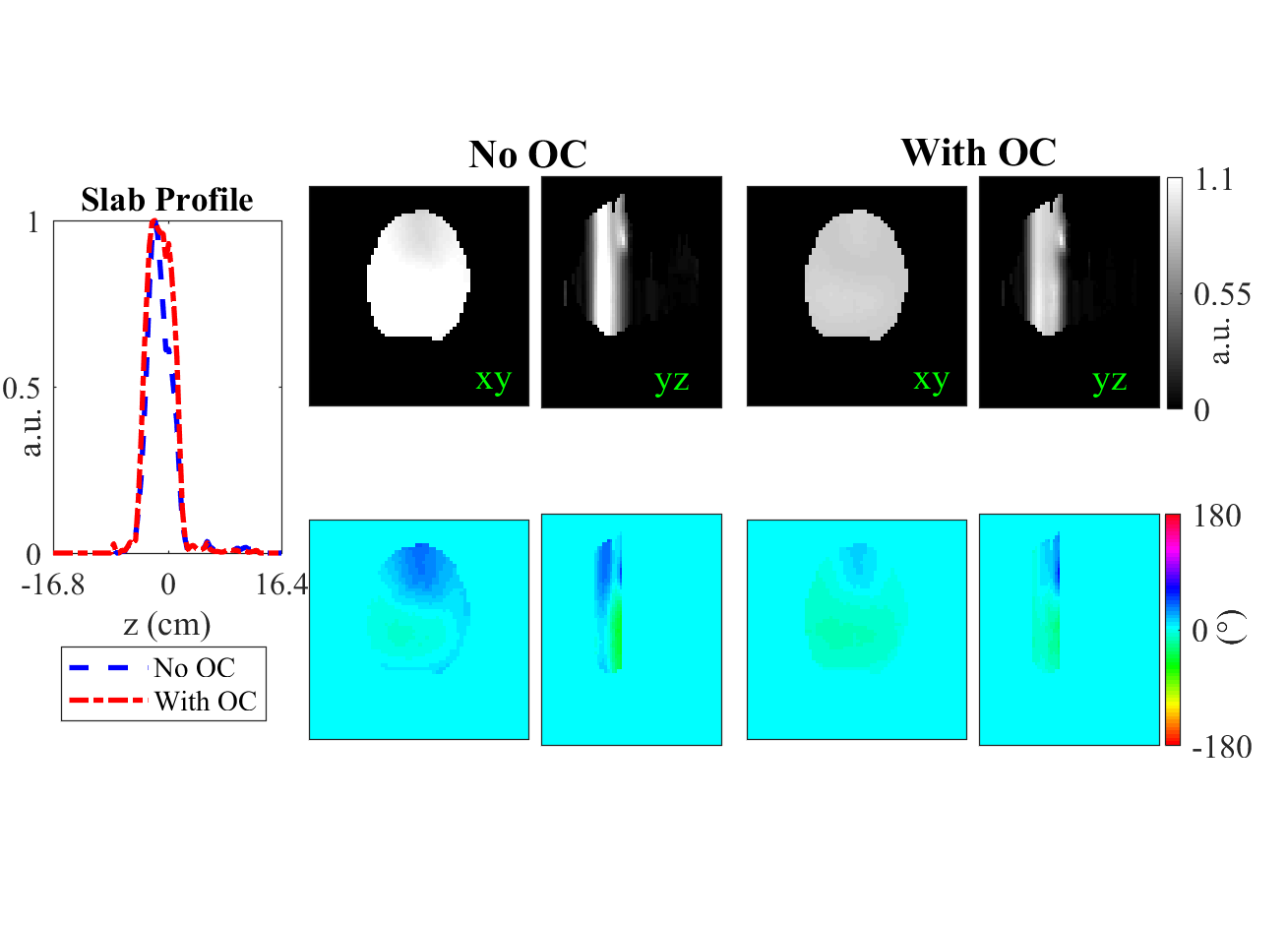
Figure 4 shows the simulated slab profile and simulated magnetization (in two imaging planes) at TE for the slab-selective prewinding pulse designed with the constrained STA and fast OC methods. At TE the magnetization magnitude should be uniform and the phase should be zero. Compared to the target prewinding pattern, the simulated magnetization from the STA/OC pulses had magnitude NRMSEs of 0.29/0.19, phase RMSEs of 22.8°/11.4° and complex NRMSEs of 0.46/0.26, respectively. The total compute time of the OC method was 55 seconds compared to the STA approach’s 24 seconds.

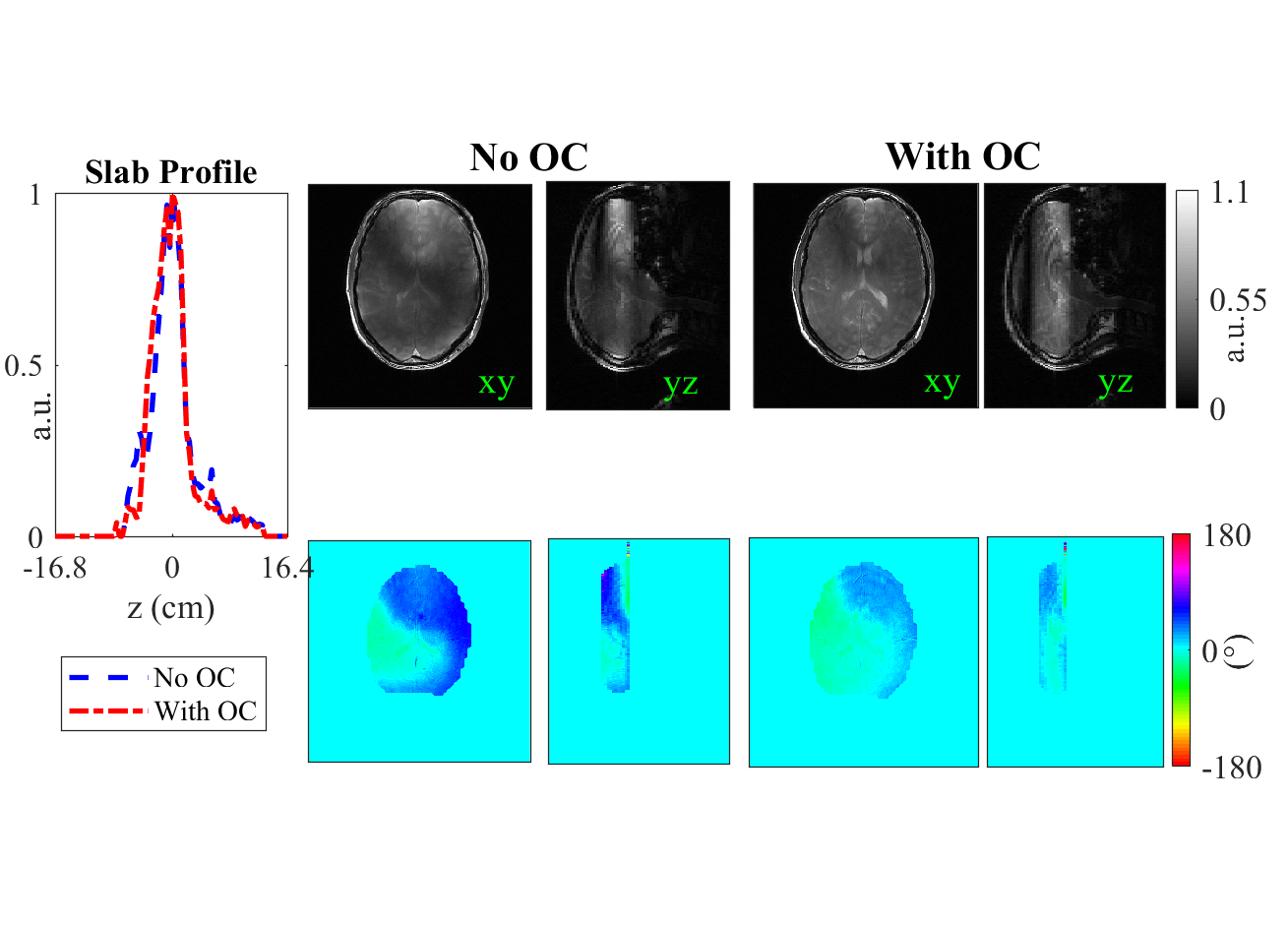
Figure 5 shows the experimental slab profiles and experimental images (in two imaging planes) for the slab-selective prewinding pulses. The slab profile is sharper and the phase image is flatter in the constrained method using the fast OC approach.

Discussion and Conclusion

Acknowledgements

References

1. Yip, C. et al., Mag. Reson. Med., 54 (4), 2005.

2. Pauly, J. et al., J. Mag. Res., 81 (1), 1989.

3. Rund, A. et al., IEEE Trans. Med. Im., 37 (2), 2018.

4. Hoyos-Idrobo, A. et al., IEEE Trans. Med. Im., 33 (3), 2014.

5. Guerin, B. et al., Mag. Reson. Med., 73 (5), 2015.

6. Conolly, S. et al., Mag. Reson. Med., 5 (2), 1986.

7. Grissom, W.A. et al., IEEE Trans. Med. Im., 28 (10), 2009.

8. Pauly, J. et al., IEEE Trans. Med. Im., 10 (1), 1991.

9. Wong, E., ISMRM, 2012.

10. Williams, S.N. et al., ISMRM, 2018.

11. Nielsen, J-F. et al., Mag. Reson. Med., 69 (3), 2013.