4620
On the Effective Centre of Excitation and the Point of Gradient Moment Expansion for 2D-Selective Excitation in the Presence of Flow1Physikalisch-Technische Bundesanstalt (PTB), Braunschweig and Berlin, Germany, 2Medical Physics in Radiology, German Cancer Research Center (DKFZ), Heidelberg, Germany, 3Working Group on Cardiovascular Magnetic Resonance, Experimental and Clinical Research Center, a joint cooperation between the Charité Medical Faculty and the Max-Delbrueck Center for Molecular Medicine, Berlin, Germany
Synopsis
In this work, we demonstrate the distinction and importance of two virtual time points during excitation for correct flow compensation and quantification: the centre of excitation ($$$t_0^\text{m}$$$) at which spins are excited and thus magnitude is generated, and the isophase time-point ($$$t_0^\text{ph}$$$) at which all excited spins are in phase. A general method to determine $$$t_0^\text{m}$$$ is presented and $$$t_0^\text{ph}$$$ and $$$t_0^\text{m}$$$ are shown to be not necessarily identical. Finally, phantom experiments demonstrate that the knowledge of $$$t_0^\text{m}$$$ is required to remove the displacement artefact in phase-encoding directions to enable correct flow compensation and imaging.
Introduction
2D-selective excitation has been employed to accelerate time-resolved flow measurements in 1D1-3 and 3D4 by reducing the field-of-view. However, applying conventional flow quantification and compensation techniques straightforwardly to 2D-selective RF-pulses can lead to a) wrong velocity quantification and b) displacement5 of moving spins possibly into static tissue.
Here, we identify for the first time two distinct virtual time-points during excitation: the isophase time-point$$$\;(t_0^\text{ph})\;$$$at which all excited spins are in phase (cf. isodelay6) and the centre of excitation$$$\;(t_0^\text{m})\;$$$at which spins are effectively excited and thus magnitude is generated. While those points coincide for standard ‘SINC’-pulses at nearly half the RF-pulse duration, their distinction is indispensable for correct flow compensation and quantification using 2D-RF-pulses:
a)$$$\;t_0^\text{ph}\;$$$is needed for correct velocity quantification and has been identified for spiral 2D-selective excitation at the 2D-RF-pulse end7,4. Here, we investigate how off-resonances affect phase and velocity quantification.
b)$$$\;t_0^\text{m}\;$$$has not been reported yet but is required to correct the displacement of moving spins caused by the time-delay between excitation and read-out in phase-encode (PE) directions.
The aim of this work is 1.) to present a general method to determine $$$t_0^\text{m}$$$, 2.) to show that$$$\;t_0^\text{ph}\;$$$and$$$\;t_0^\text{m}\;$$$are not necessarily identical, and 3.) to demonstrate in phantom experiments that precise knowledge of$$$\;t_0^\text{m}\;$$$is required to remove the displacement artefact in PE-directions.
Theory
In MR flow imaging, velocity is quantified by using bipolar gradients$$$\;\boldsymbol{G}(t)\;$$$that impart a velocity dependent phase to the spins$$\phi=\gamma(\boldsymbol{r}\cdot\boldsymbol{m}_0+\boldsymbol{v}\cdot\boldsymbol{m}_1+\cdot\cdot\cdot).$$This equation results from a Taylor expansion around the expansion time-point$$$\;t_\text{exp}$$$8. Here,$$$\;\boldsymbol{r}\;$$$and$$$\;\boldsymbol{v}\;$$$denote the spin’s position and velocity at$$$\;t_\text{exp}$$$, while$$$\;\gamma\;$$$denotes the gyromagnetic ratio. The zeroth and first gradient moment at echo time$$$\;t_\text{TE}$$$ $$\boldsymbol{m}_0=\int_{t_0}^{t_\text{TE}}\boldsymbol{G}(\tau)\text{d}\tau$$ $$\boldsymbol{m}_1=\int_{t_0}^{t_\text{TE}}\boldsymbol{G}(\tau)(\tau-t_\text{exp})\text{d}\tau$$are calculated starting from the pulse's isophase timepoint,$$$\;t_0=t_0^\text{ph}$$$, when all spins are phase aligned. Thus,$$$\;t_0^\text{ph}\;$$$is essential to design velocity encoding gradients. Since position and velocity are encoded at$$$\;t_\text{exp}$$$, a spatial shift (displacement) of the spins $$\Delta\boldsymbol{r}=\boldsymbol{v}\cdot(t_\text{exp}-t_0^\text{m})$$ will be observed, if$$$\;t_\text{exp}\neq\,t_0^\text{m}\;$$$for designing bipolar gradients. While setting$$$\;t_\text{exp}=t_0^\text{m}\;$$$will remove the shift along PE directions, it cannot be compensated along read-out (RO), since$$$\;m_1^\text{RO}\;$$$varies during data acquisition9.Methods
2D-selective excitation
Two 3.5ms long 2D-selective RF-pulses with spiral k-space trajectory were designed7 as described in4 to excite a rectangular bar with 1) a large field-of-excitation FOX=$$$(\infty\times60\times60)\,\text{mm}\;$$$and bandwidth-time-product BWT=1.2 (RFL) and 2) a small FOX=$$$(\infty\times36\times36)\,\text{mm}\;$$$and BWT=0.9 (RFS).
Simulations
The velocity-dependent phase of the magnetisation at the 2D-RF-pulse end$$$\;T_\text{end}\;$$$was determined using Bloch-simulations. Additionally, the impact of off-resonance on velocity quantification was investigated by simulating the 2D-RF-pulses once with consecutive flow-encoding and second with flow-compensation gradients. Simulated spins move in a virtual tube oriented in $$$y$$$-direction (PE) with maximum velocities $$$v_y\in[-100:20:100]\,\text{cm}/\text{s}$$$ and are static elsewhere.
The location of $$$t_0^\text{m}$$$ was quantified by evaluating the spatial shifts of the magnitude pattern at $$$T_\text{end}$$$ in Bloch-simulations using moving spins in comparison to stationary spins. The spatial shift of the magnitude signal $$$|S(y,v_y)|$$$ was calculated by $$$\Delta y=\frac{\int|S(y,v_y)|\,y\,\text{d}y}{\int|S(y,v_y)|\text{d}y}$$$ for $$$v_y\in[-100:20:100]\,\text{cm}/\text{s}$$$ and RFS and RFL. The centre of excitation is then calculated by $$$t_0^\text{m}=T_\text{end}-\frac{\Delta y}{v_y}$$$.
Experiments
Flow phantoms containing two pipes with constant flow were scanned at 3T (Magnetom Verio, Siemens) using a 15-channel-knee-coil to verify the simulation results. RFL- and RFS-excitation pattern shifts were measured for $$$t_\text{exp}=t_0^\text{ph}$$$, $$$t_\text{exp}=t_0^\text{m}$$$, and $$$t_\text{exp}=t_\text{TE}$$$ in the presence and absence of flow. Imaging parameters of two datasets differing mainly in venc: dataset1/dataset2: venc(z)=2m/s/4.5m/s, TE=3.35ms/3.25ms, FA=8°/3°, matrix=64x64x192/96x96x192, resolution=2x2x1mm3/1.5x1.5x1mm3. Receive profiles were eliminated using separate acquisitions with non-selective excitations.
Results
Simulations
Since$$$\;t_0^\text{ph}=T_\text{end}\;$$$for moving spins and zero off-resonance4, phase at$$$\;T_\text{end}\;$$$is velocity-independent (Fig.1a). However, for 200 and 500Hz off-resonance, phase is varying non-linearly as a function of velocity (Fig.1b). Still, the same velocity is quantified for zero and 200Hz off-resonance (Fig.2a,bottom). Actually, a fit shows that quantified$$$\;v_\text{qu}\;$$$and actual velocity$$$\;v_\text{act}\;$$$match for 0 and 200Hz off-resonance (Fig.2b) with fit difference close to zero (Fig.2c).
The magnitude pattern is smoothened for 200Hz off-resonance and shifted in the moving tissue section (Fig.2a,top). Figure3 depicts the shift of the RFL- and RFS-excitation patterns at $$$T_\text{end}$$$ for different velocities along y-direction. Based on this velocity-dependent shift the magnitude’s centre of excitation was located before$$$\;T_\text{end}$$$ at $$$T_\text{end}-t_0^\text{m}=(0.52\pm0.01)\,\text{ms}$$$ and $$$(0.75\pm0.02)\,\text{ms}$$$ for RFL and RFS respectively, while $$$t_0^\text{ph}$$$ was identified at $$$T_\text{end}$$$.
Experiments
Figure4 illustrates that the flow-induced excitation pattern shift of up to $$$12.5\,\text{mm}\,$$$for$$$\;t_\text{exp}=t_\text{TE}\;$$$and$$$\;v=2.9\,\text{m}/\text{s}\;$$$is successfully suppressed choosing$$$\;t_\text{exp}=t_0^\text{m}$$$. Figure5 shows the RFL- and RFS-shift for different velocities and$$$\;t_\text{exp}$$$. The measurements agree with simulations predicting $$$\Delta\boldsymbol{r}=\boldsymbol{v}\cdot(t_\text{exp}-t_0^\text{m})$$$ and thus zero shift for $$$t_\text{exp}=t_0^\text{m}$$$.
Discussion and Conclusion
In this work, for the first time, distinct excitation time-points for phase$$$\;t_0^\text{ph}\;$$$and magnitude$$$\;t_0^\text{m}\;$$$are identified for velocity-encoding and compensation. Although off-resonances distort the magnitude pattern and phase varies non-linearly with velocity, flow quantification remains granted. Nevertheless, precise knowledge of$$$~t_0^\text{m}~$$$is essential to suppress the
flow-induced displacement artefact in PE-direction. While these findings were derived for 2D-selective RF-pulses, ongoing work suggests them being similarly important for asymmetric 1D-selective excitation pulses, like minimum-phase Shinnar-Le-Roux-pulses10.Acknowledgements
No acknowledgement found.References
1. Hardy CJ, Pearlman JD, Moore JR, Roemer PB, Cline HE. Rapid NMR Cardiography with a Half-Echo M-Mode Method. Journal of Computer Assisted Tomography. 1991
2. Butts K, Hangiandreou NJ, Riederer SJ. Phase velocity mapping with a real time line scan technique. Magnetic Resonance in Medicine. 1993;29(1):134–138.
3. Hardy CJ, Darrow RD,
Nieters EJ, Roemer PB, Watkins RD, Adams WJ, et al. Real-time acquisition,
display, and interactive graphic control of NMR cardiac profiles and images.
Magnetic Resonance in Medicine. 1993;29(5):667–673.
4. Wink C, Ferrazzi G, Bassenge JP, Flassbeck S, Schmidt S, Schaeffter T, Schmitter S. 4D flow imaging with reduced field-of-excitation. Proceedings of the 27th Annual Meeting ISMRM. 2018.
5. Nishimura DG, Jackson JI, Pauly JM. On the Nature and Reduction of the Displacement Artifact in Flow Images. Magnetic Resonance in Medicine. 1991;22:481-492.
6. Bernstein MA, King KF, Zhou XJ. Handbook of MRI pulse sequences. Glover GH, editor. John Wiley & Sons, Ltd; 2005.
7. Pauly J, Nishimura D, Macovski A. A k-space analysis of small-tip-angle excitation. Journal of Magnetic Resonance (1969). 1989;81(1):43 – 56.
8. Simonetti OP, Wendt RE, Duerk JL. Significance of the point of expansion in interpretation of gradient moments and motion sensitivity. Journal of Magnetic Resonance Imaging. 1991;1(5):569–577.
9. Schmidt S, Flassbeck S, Ladd ME, Schmitter S. On the Point of Gradient Moment Expansion for Multi-Spoke RF Pulses. Proceedings of the 27th Annual Meeting ISMRM. 2018.
10. Pauly J, Le Roux P, Nishimura D, Macovski A. Parameter relations for the Shinnar-Le Roux Selective Excitation Pulse Design Algorithm. IEEE Transactions on Medical Imaging. 1991;10:53-65.
Figures
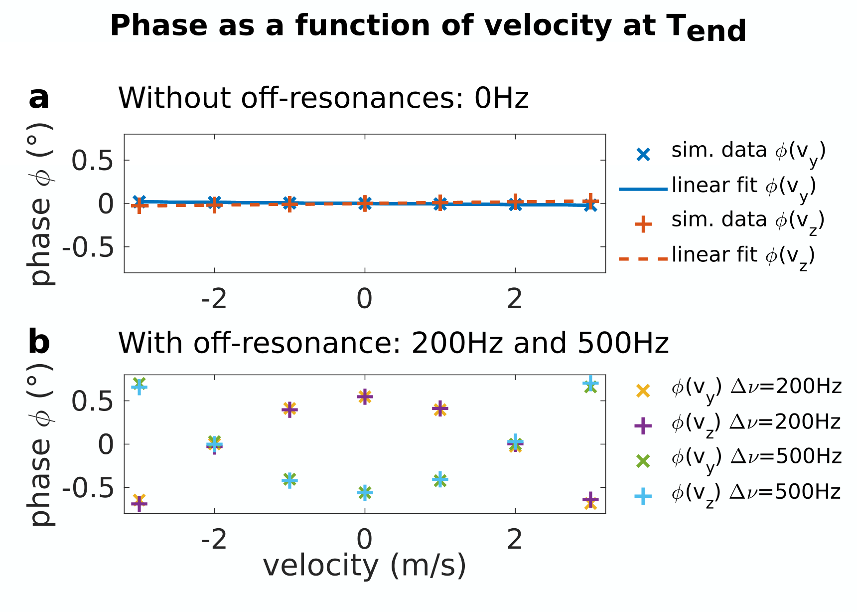
Figure 1:
The transverse magnetisation's phase as a function of spin velocity for (a) zero and (b) 200Hz and 500Hz off-resonance.
(a) Since $$$t_0^{\text{ph}}=T_\text{end}$$$ for moving spins and zero off-resonance4, the phase at $$$T_\text{end}$$$ is nearly independent of velocity and can be linearly fitted.
(b) For 200Hz and 500Hz off-resonance, the phase varies non-linearly as a function of velocity. However, the effects of off-resonance on phase are small and flow quantification is not severly impeded as shown in Fig.2.
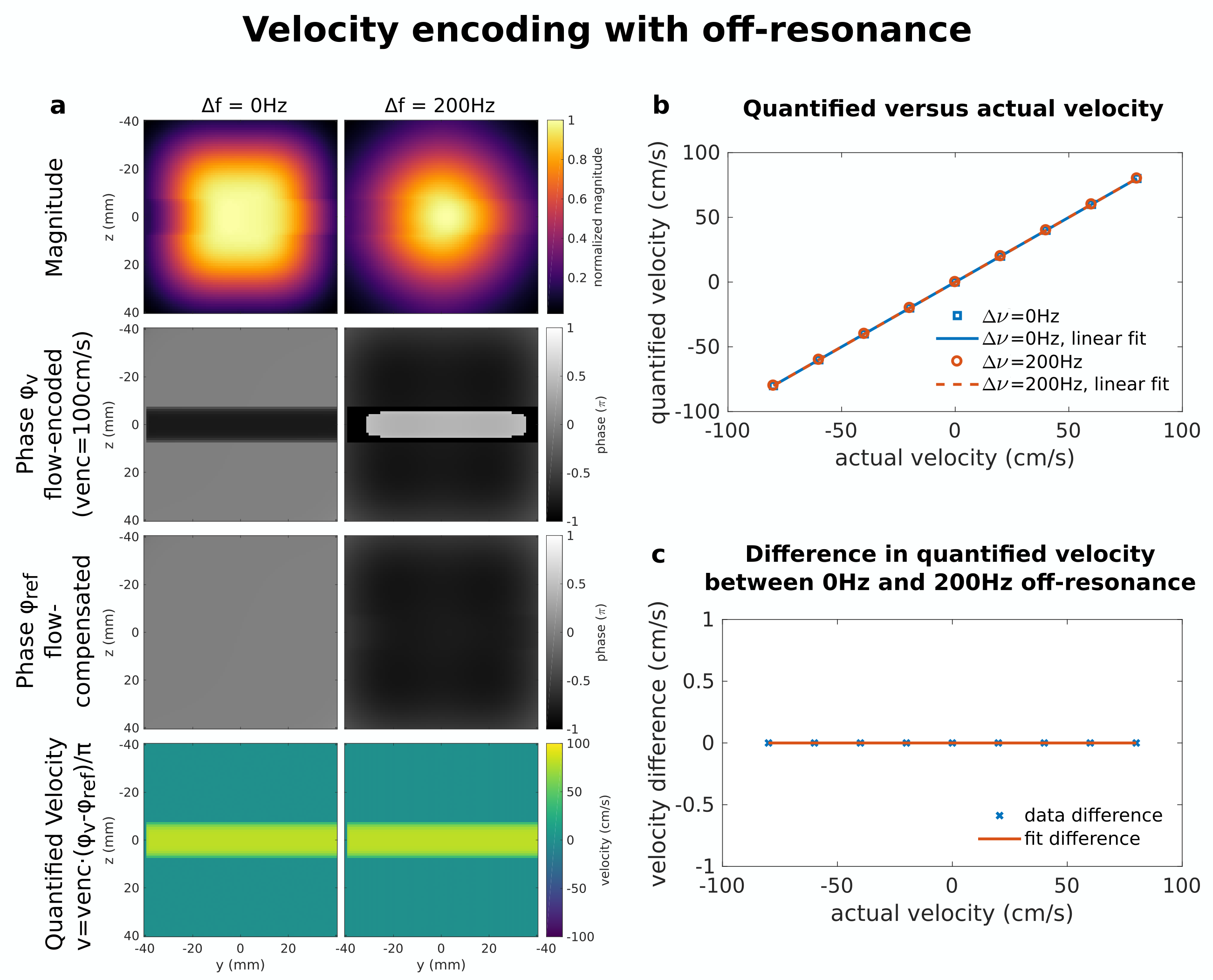
Figure 2:
Results of Bloch simulations of RFL and consecutive flow-encoding or -compensation gradients for 0Hz and 200Hz off-resonance. Spins move in y-direction with maximal$$$\;v_y=80\,\text{cm}/\text{s}$$$ in the centre of the tube.
(a) Magnitude images (1st row) exhibit the apparent displacement of the moving tissue section. Corresponding flow-encoded (2nd row:$$$~m_1=11.74\,\frac{\text{mT}}{\text{m}}\text{ms}^2$$$) and flow-compensated (3rd row:$$$~m_1=0\,\frac{\text{mT}}{\text{m}}\text{ms}^2$$$) phase images, resulting in $$$v_\text{enc}=100\,\text{cm}/\text{s}$$$. The 4th row shows the quantified velocity.
(b) Quantified versus actual velocity for off-resonances of 0Hz (blue squares) and 200Hz (red circles) for different velocities.
(c) Difference in quantified velocity between 0Hz and 200Hz off-resonance (blue 'x') and the respective fit difference (red line), which is $$$<10^{-12}\,\text{cm}/{\text{s}}$$$.
Figure 3 (animated):
(column1&2) 2D and 1D cross-section of the excitation pattern at the end of excitation $$$T_\text{end}$$$ for velocities $$$v\in[-100,100]\text{cm}/\text{s}$$$ and 2D RF-pulse RFL (left) and RFS (right). The dashed line indicates the respective shift of the excitation pattern $$$\Delta y$$$.
(column3) The 1st row shows the excitation pattern shift $$$\Delta y$$$
versus velocity $$$v_y$$$ for pulse RFL (filled blue squares) and RFS (red
circles). The 2nd row shows the resulting time
$$$T_\text{end}-t_0^\text{m}=\Delta y/v_y$$$ as a function of velocity.
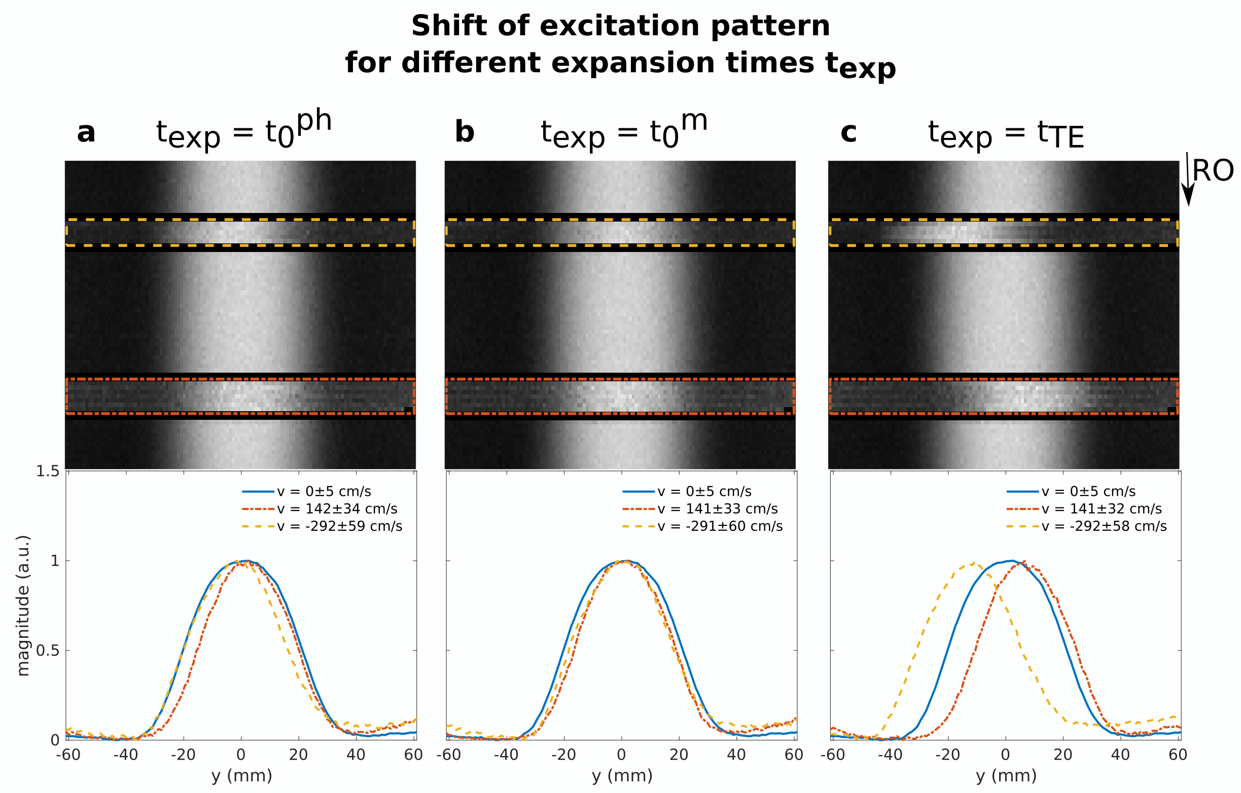
Figure 4:
(top) Magnitude images obtained using 2D-selective excitation (RFS) in a flow phantom with two pipes. RO is oriented along the non-selective axis perpendicular to the flow direction.
(bottom) The lineplots show the normalized mean magnitude in the tubes containing flowing (red & yellow) or static water (blue).
(a) Setting the expansion point $$$t_\text{exp}=t_0^\text{ph}=T_\text{end}$$$, excitation pattern shifts of -1.70±0.32 mm and 1.23±0.03mm are observed.
(b) Setting $$$t_\text{exp}=t_0^\text{m}=T_\text{end}-0.75\,\text{ms}$$$, these shifts are well compensated for both flow directions and velocities with residual displacements of 0.26±0.21mm and -0.18±0.03mm.
(c) Setting $$$t_\text{exp}=t_\text{TE}=T_\text{end}+3.25\,\text{ms}$$$ even higher shifts of -12.49±0.22mm and 5.70±0.09mm are observed.
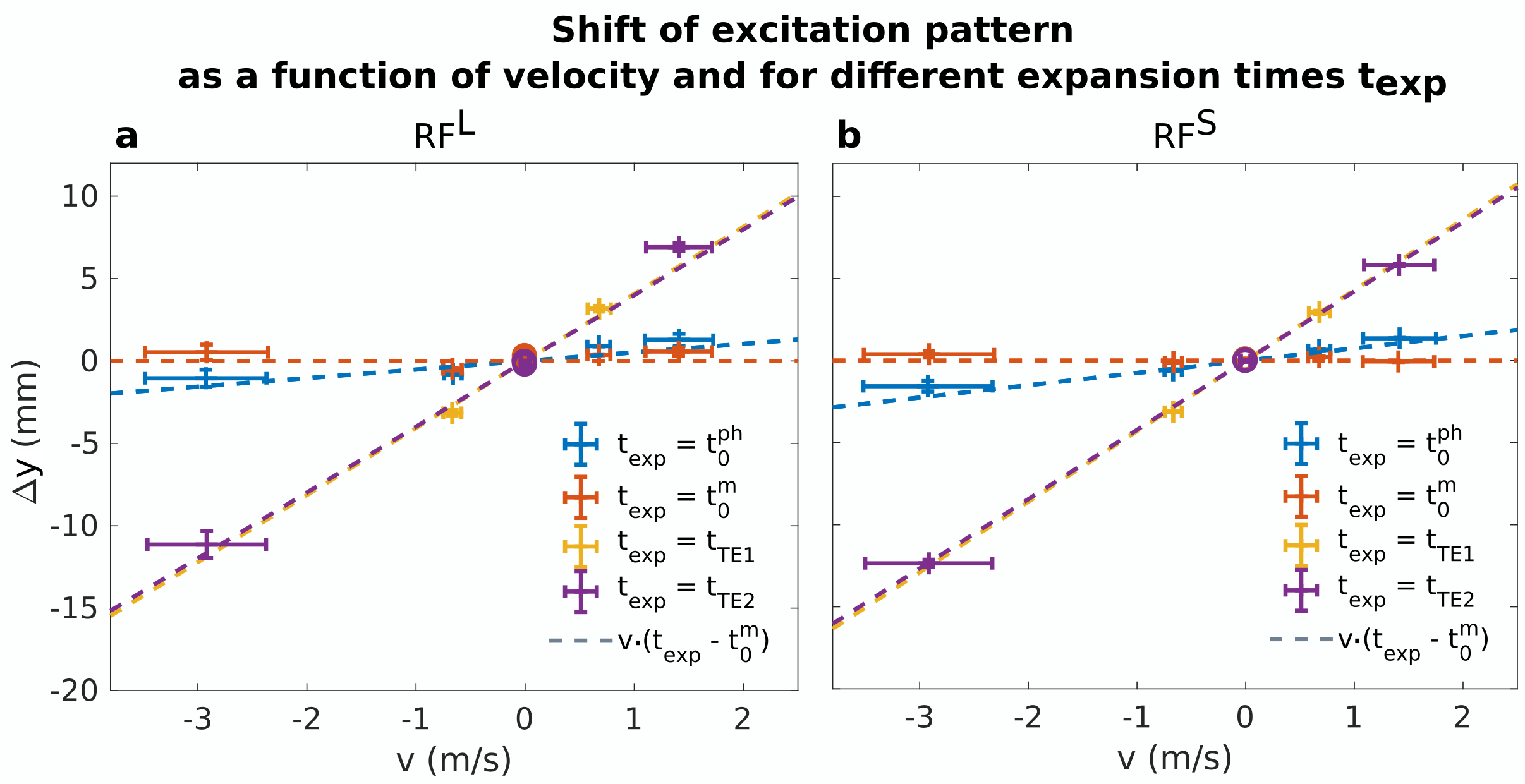
Figure 5:
The measured, offset-corrected mean shift of the 2D-selective excitation
pattern (a: RFL, b: RFS) as a function of velocity for different choices of
$$$t_\text{exp}$$$. The dashed lines indicate the expected shift $$$\Delta y=v_y\cdot(t_\text{exp}-t_0^\text{m})$$$. Yellow and violet data points were obtained using venc settings of venc1=2m/s and venc2=4.5m/s that led to different echo times of TE1=3.35ms and TE2=3.25ms.
While all other settings of $$$t_\text{exp}$$$ result in displacements scaling linearly with flow velocity and the deviation of $$$t_\text{exp}$$$ from $$$t_0^\text{m}$$$, these artefacts are successfully suppressed for all velocities if $$$t_\text{exp}=t_0^\text{m}$$$ (red symbols) is chosen for calculating bipolar gradients.